XYZ: gapped spinons and bound branches¶

View this page on GitHub

The XYZ chain is a useful next step beyond XXZ for an excitation ansatz: it has domain walls, bound excitations and discrete symmetry labels, but no conserved total \(S^z\). This tutorial shows how to specify the couplings and compare its thermodynamic lines without confusing a momentum copy with a new particle or a continuum envelope with an operator-resolved spectrum.

1. Turn the input parameters into physical couplings¶

The frontend uses two elliptic parameters, --eta and --t, and an overall energy scale --exchange J:

\[ H=J\sum_j\left(J_x S_j^xS_{j+1}^x+J_y S_j^yS_{j+1}^y+J_z S_j^zS_{j+1}^z\right). \]

These are spin-1/2 operators, \(S=\sigma/2\), at zero field and temperature. The dimensionless couplings \(J_x,J_y,J_z\) are theta-function ratios, defined in the reference guide. t is a theta parameter, not time, temperature or hopping. eta is not an XXZ anisotropy that can be substituted directly for \(\Delta\).

Start with:

bethe-xyz-dispersion --eta 0.75 --t 1 --points 129
bethe-xyz-dispersion --eta 0.75 --t 1 --points 129 \
  --precision fp64 --format csv > xyz.csv

The exported metadata gives the actual couplings. For the examples here, \(t=J=1\):

eta	Jx	Jy	Jz	Download
0.4	1.171134	0.856085	0.306933	CSV
0.5	1.189207	0.840896	0	CSV
0.75	1.094588	0.920435	−0.704471	CSV

Use the full-precision metadata for numerical comparisons; the table is rounded for readability. Varying eta changes several couplings together. This frontend covers the region \(J_x\gt J_y\gt|J_z|\), not arbitrary exchange triples or a general coupling-inversion problem.

2. A single spinon is a domain wall¶

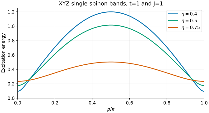
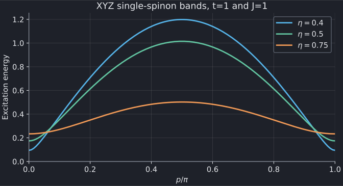
Single-spinon bands at three elliptic parameters

The ordered chain has two x-Néel vacua. A single spinon connects different vacua at its two ends; its energy is appropriate for a domain-wall excitation ansatz. It is not the lowest local excitation within one fixed vacuum.

The curve has the form

\[ \epsilon(p)=\sqrt{m^2\cos^2p+I^2\sin^2p},\qquad 0\le p\le\pi, \]

where the metadata supplies the single-spinon gap \(m\) and band maximum \(I\). The plot reads the frontend's energies rather than reconstructing them from this formula. Our tests use the formula as a separate consistency check.

The middle example, eta=0.5, is an anisotropic XY chain with \(J_z=0\). It is still gapped because \(J_x\ne J_y\). The independent XY relations \(m=J(J_x-J_y)/2\) and \(I=J(J_x+J_y)/2\) provide a useful normalization test.

Changing only --exchange multiplies all energies by the same factor and leaves momenta and dimensionless couplings unchanged. The saved J=2 export checks this against the eta=0.75 example.

3. Select a bound branch—and check that it exists¶

A positive integer index \(s\) is present only when

\[ s(1-\eta)\lt\eta. \]

At eta=0.75, the allowed indices are 1 and 2. Index 3 sits exactly at a merger and is excluded. At eta=0.5, even index 1 is at its merger: there is no isolated bound branch. --branch all omits nonexistent branches; a bound-only request in a region without one is an input error.

bethe-xyz-dispersion --eta 0.75 --t 1 --branch bound --bound-state 1

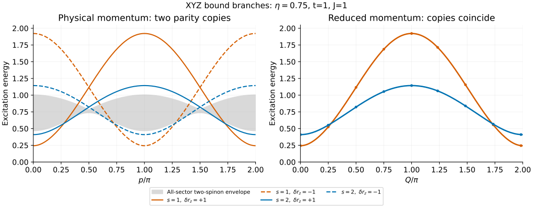
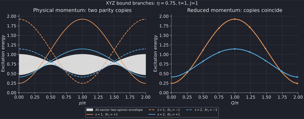
Physical and reduced momentum views of both bound branches

Each bound index appears in two relative z-parity channels. Their physical momenta differ by pi, but their reduced-momentum dispersions coincide:

\[ \delta r_x=(-1)^s,\qquad \delta r_z=\pm1,\qquad Q=p-\pi\frac{1-\delta r_z}{2}\pmod{2\pi}. \]

The left panel uses p, with solid and dashed curves for the two z-parity copies. The right uses reduced_q; the dashed curves with markers lie on their solid partners. These are parity ratios relative to a chosen vacuum, not absolute parity labels of a finite ring. Do not assign \(S^z\) labels to generic XYZ branches.

For a two-site MPS cell the translation phase is \(k_{\mathrm{cell}}=2p\pmod{2\pi}\). It agrees for corresponding points in the two copies. It is not the same coordinate as \(Q\), and folding momentum does not erase their discrete symmetry labels.

4. Interpret the continuum shading carefully¶

The grey region is the exported all-sector two-spinon envelope, including pi-shifted translation copies. It is not resolved by parity and does not supply spectral weights. An excitation in a particular operator channel need not see every scattering state inside it.

At eta=0.75 and \(Q=0\), the first two bound gaps are approximately 0.243787 and 0.409824, below \(2m\simeq0.466366\). The single-spinon gap is smaller, \(m\simeq0.233183\), but belongs to a different asymptotic-vacuum sector. These are three different quantities—not alternative estimates of one gap.

Elsewhere a bound curve can lie inside or above the all-sector envelope. “Bound” does not mean below that envelope at every physical momentum. Neither overlap nor its absence in this plot determines a decay rate or an operator's spectral intensity.

Also, these are thermodynamic formulas. Finite-ring parity partners can split, and the nearly degenerate ground-state combinations have a finite-size splitting of their own. Neither effect is included in this plot. See the reference guide's finite-size checks before comparing with a short periodic MPS.

5. Reproduce and check¶

With the optional plotting environment:

python3 scripts/plot_xyz_tutorial.py
# Regenerate the four frontend exports too:
python3 scripts/plot_xyz_tutorial.py \
  --solver bethe-xyz-dispersion
python3 scripts/plot_xyz_tutorial.py --check
python3 -m unittest discover -s scripts -p 'test_tutorial_xyz.py'

The checks cover every branch grid, nullable columns, status, momentum shift, parity, strict merger condition, XY limit and exchange scaling. Failed rows must stay missing, not become zero-energy lines. Native long-double and fp128 are available where supported; exceptionally small gaps can require more range or precision than the fp64 examples used here.