Sutherland: the collision rule is part of the model¶

View this page on GitHub

Can two Bose gases with a vanishing explicit potential have different spectra? Yes: their allowed wavefunctions can obey different rules at particle coincidences. The Sutherland model makes this distinction unusually concrete. We will compare three collision exponents, identify a few excitations by their integer labels, and see what a finite spectrum scan does—and does not—cover.

This is the scalar continuum inverse-square gas, not the SU(3) Uimin–Lai– Sutherland spin chain. For that model, see the ULS tutorial.

1. Specify the Hamiltonian and its collision branch¶

With \(\hbar=2m=1\), periodic length \(L\) and \(\lambda\geq0\):

\[ H=-\sum_j\partial_{x_j}^2+ 2\lambda(\lambda-1)\left(\frac{\pi}{L}\right)^2 \sum_{i\lt j}\frac{1}{\sin^2[\pi(x_i-x_j)/L]}. \]

Our solver selects periodic bosonic wavefunctions with collision behaviour \(\Psi\sim|x_i-x_j|^\lambda\). Thus --lambda specifies more than the coefficient of the potential:

\(\lambda=0\): free bosons, with no forced zero at coincidence.
\(\lambda=1\): hard-core bosons, with a zero at coincidence—even though the displayed potential coefficient is again zero.
\(\lambda=2\): a stronger collision zero and a nonzero repulsive potential.

In particular, replacing \(\lambda\) by \(1-\lambda\) leaves the potential coefficient unchanged but generally changes the collision branch. A coupling coefficient alone is not a complete specification of this singular Hamiltonian.

2. Compare a small ring¶

Use four particles on a ring of length four and enumerate a small label window:

bethe-sutherland-pbc 4 --length 4 --lambda 1 --levels all --window 1
bethe-sutherland-pbc 4 --length 4 --lambda 1 --levels all --window 1 \
  --precision fp64 --format csv > sutherland-lambda1.csv

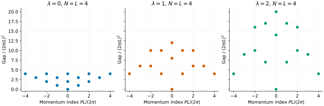
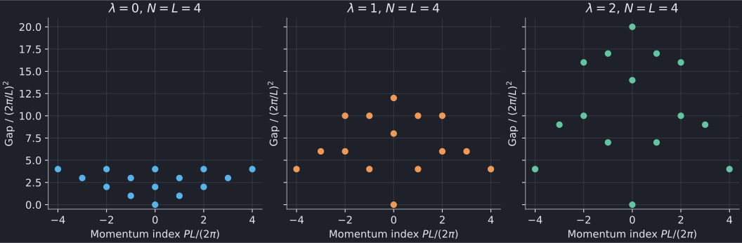
Excitation gaps for collision exponents zero, one and two

Each panel uses an actual frontend export: lambda = 0, lambda = 1, lambda = 2. The vertical axis is the gap above each model's own ground state, in units of \(q^2\), where \(q=2\pi/L\). The horizontal axis is the integer \(P/q\), not a momentum reduced to a Brillouin zone.

The ground-state energies differ as well:

\[ E_0=\left(\frac{\pi}{L}\right)^2 \frac{\lambda^2 N(N^2-1)}{3}. \]

For this ring, \(E_0/q^2=5\lambda^2\). In particular, hard-core and free bosons differ both in ground energy and in many excitation gaps despite the zero explicit potential coefficient in both cases.

3. Read a state label¶

A state has \(N\) ascending integer labels \(n_0,\ldots,n_{N-1}\). Repeated and negative labels are allowed. The ground state has all labels zero. The pseudomomenta and observables are

\[ k_j=q\left[n_j+\lambda\left(j-\frac{N-1}{2}\right)\right], \qquad P=q\sum_j n_j,\qquad E=\sum_j k_j^2. \]

The pseudomomenta need not be single-particle orbital momenta. The collision rule is already encoded in their spacing.

Two useful excitations at \(N=4\) are:

Labels	\(P/q\)	\((E-E_0)/q^2\)	Interpretation
`0 0 0 1`	1	\(1+3\lambda\)	Raise the largest label
`1 1 1 1`	4	4	Boost the whole ground state

The first gap depends on the collision exponent; the common boost costs the same amount for all three exponents. You can select a state directly:

bethe-sutherland-pbc 4 --length 4 --lambda 2 --labels 0,0,0,1

Doubling \(L\) at fixed particle number, exponent and labels halves all momenta and quarters all energies. The saved length-eight export checks that scaling. This is a finite-size change at fixed \(N\), not a thermodynamic limit at fixed density.

4. What does “all” mean?¶

--levels all --window 1 includes all ascending labels drawn from -1, 0, 1: fifteen states for four particles. It does not mean every excitation of the model. The full spectrum is infinite.

Enlarge the window:

bethe-sutherland-pbc 4 --length 4 --lambda 1 --levels all --window 2 \
  --precision fp64 --format csv > sutherland-window2.csv

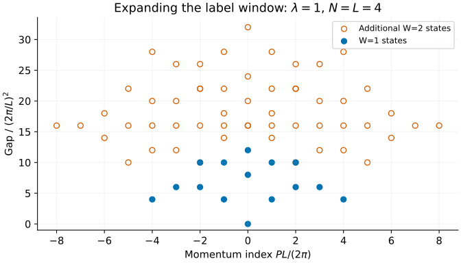
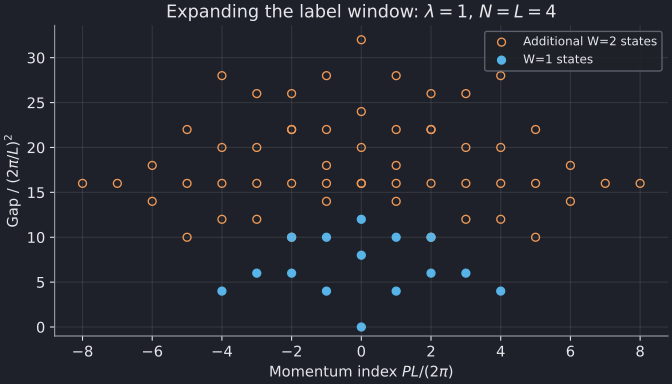
States added by enlarging the label window from one to two

The larger export contains seventy states. Blue points are the original window; orange rings mark additional label sequences. Several distinct states can share a plotted energy and momentum, so the number of visible dots is not the state count.

For a symmetric window \([-W,W]\), the number of label sequences is

\[ \binom{N+2W}{N}. \]

It grows quickly. --levels COUNT limits the output but still searches the specified window; --max-states guards the enumeration size. A successful scan certifies coverage inside that window, not a globally complete low-energy spectrum. Never silently interpret a truncated scan as an absence of states elsewhere.

5. Use this as a numerical benchmark¶

The solver applies exact spectral rules, evaluated in the selected floating- point precision. The CSV status exact spectral rules does not mean infinite- precision arithmetic. fp64 is the default; long-double, configured fp128 and explicit MPFR are also available. The saved examples retain their original arithmetic.

For a continuum MPS or a discretized calculation, check the collision branch as carefully as the written potential. A naive zero-potential discretization does not enforce the hard-core branch automatically. Compare gaps at matched particle number and circumference, and do not fold these physical continuum momenta as if there were an underlying lattice.

These tables contain energies and momenta, not wavefunctions, form factors or spectral weights. The reference guide gives the domain conventions, numerical limits and further state-selection examples.

6. Reproduce and check¶

With the optional plotting environment:

python3 scripts/plot_sutherland_tutorial.py
# Also regenerate the five saved exports:
python3 scripts/plot_sutherland_tutorial.py \
  --solver bethe-sutherland-pbc
python3 scripts/plot_sutherland_tutorial.py --check
python3 -m unittest discover -s scripts -p 'test_tutorial_sutherland.py'

The checks verify every label in the accepted window, momentum units, energy references, length scaling, reflection symmetry and the two explicit gaps above. Failed aggregate status or missing states are rejected even though this exact-rule frontend has no iterative status column on each row.