Integrable ladder: reconstruct a finite-size magnetization curve
All tutorials · Model guide · SU(3)/ULS tutorial
This example uses fixed-magnetization energies to build a field-dependent ground-state envelope. It also explains why a ladder's physical singlet/triplet populations are not always the highest-weight labels of its Bethe roots.
1. Include the required four-spin interaction
This is Wang's integrable ladder, not the ordinary two-leg Heisenberg ladder. There are L rungs, each with two spin-1/2 operators S and T:
The coefficients 1,1,4 are fixed. The field has the usual negative Zeeman sign, and translation is by one rung, not one spin. Periodic L=2 counts the closing bond separately. Arbitrary four-spin coefficients and open ends are not implemented.
A rung has one singlet s and three triplets t+,t0,t-. Its leg interaction equals a four-color permutation minus 1/4, so
The energy constants matter when comparing an MPO to the solver. M is total magnetization, not M/L. The paper's permutation convention uses J_r=2J; our guide restores the physical ladder constants above.
2. Obtain one energy per total-Sz sector
Choose six rungs and J_r=5. For example, the M=2 calculation is
bethe-ladder-pbc 6 --rung 5 --sz 2 \
  --csv-table states=ladder-m2.csv \
  --csv-table representations=ladder-representations.csv \
  --csv-table roots=ladder-roots.csv
It minimizes the singlet count and triplet populations compatible with M=2, giving N_s=4 and energy -15.23606798. Repeating for M=0,…,6 yields:
| M | Minimizing N_s | E at h=0 |
|---|---|---|
| 0 | 6 | -18 |
| 1 | 5 | -17 |
| 2 | 4 | -15.23606798 |
| 3 | 3 | -11.60555128 |
| 4 | 2 | -5.23606798 |
| 5 | 1 | 3 |
| 6 | 0 | 12 |
At fixed M, h only adds -hM: it does not change the minimizing roots or N_s. Negative-M zero-field energies follow by spin reversal. These are minima of Sz sectors, not prescribed total-spin S and not excited-state enumeration.
3. Take the minimum of the linear branches
For positive h, construct
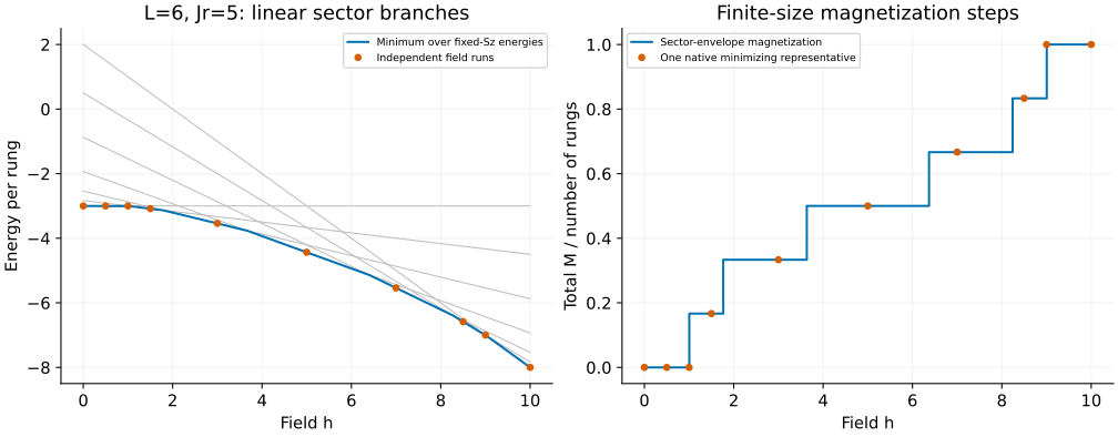
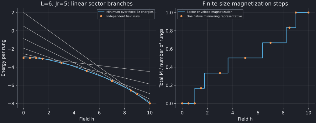
The grey lines use the seven native zero-field energies; the blue curve is
their minimum. Orange markers are separate native field calculations
without --sz, for example:
bethe-ladder-pbc 6 --rung 5 --field 3
At h=3 this returns M=2 and E=-21.23606798. The second panel divides total M by L. For these data every M appears; in general, some finite-size sectors can be skipped by the lower envelope and must not be forced into a staircase.
Adjacent crossings here occur at h approximately 1, 1.76393202, 3.63051670, 6.36948330, 8.23606798 and 9. Exactly at a crossing the magnetization is not unique. At h=9 the native analytic path returns M=6, while the plotting envelope's tie rule selects M=5; both have E=-42. This is a choice of degenerate representative, not a disagreement or a thermal average.
The all-singlet product has \(E_s=3L(1-J_r)/4\). It is a ground state whenever J_r-|h|≥4; the fully polarized triplet product is a ground state when |h|≥4+max(J_r,0). These sufficient bounds explain the outer parts of this example, not every finite-ring transition in every parameter regime.
The minimum one-triplet cost above the singlet product is
At J_r=5,h=0 this gives 1 for L=6 but approximately 1.38196601 for L=5. The odd ring cannot put the triplet exactly at momentum π. Both cases are included as native finite-size checks; there is no thermodynamic extrapolation hidden in the field plot.
4. Do not identify physical populations with root labels
Now change to J_r=0 and constrain four singlet rungs:
bethe-ladder-pbc 6 --rung 0 --singlets 4 --roots
The report distinguishes two vectors:
| Meaning | Four entries |
|---|---|
| Physical populations (s,t+,t0,t-) | (4,1,1,0) |
| SU(4) highest-weight rows | (4,2,0,0) |
The physical state is a descendant of the latter multiplet. Its permutation energy is \(1-\sqrt5\) and physical ladder energy is \(-1/2-\sqrt5\simeq-2.73606798\). Solving only the packed sea of the physical population's own highest weight would instead give permutation energy -1, missing the lower state. The frontend compares compatible highest weights.
Only the highest-weight representative's finite roots are exported. Lowering operators change populations without changing that permutation energy; the program does not fabricate finite roots for the descendant.
At zero field the displayed triplets are a balanced representative with M=1, not a unique magnetization. An arbitrarily small positive field selects M=2 inside this multiplet: at h=0.125 the populations are (4,2,0,0), and the energy drops by 0.25, not 0.125. Negative h swaps t+ and t-. The saved examples also shift J_r from 0 to 1 at fixed N_s=4, lowering E by 2.5 without changing the representative roots.
This matters for symmetry-aware MPS comparisons: match physical M and N_s, use rung momentum, and keep the highest-weight label separate. An incomplete scan reports a candidate upper bound, not a completed sector minimum. Convergence of this real-sea ground-state construction is not a general completeness theorem for all nested Bethe eigenstates.
5. Reproduce and validate
Each calculation has three native tables:
| Fixed M, J_r=5,h=0 | State | Representations | Roots |
|---|---|---|---|
| 0 | CSV | CSV | CSV |
| 1 | CSV | CSV | CSV |
| 2 | CSV | CSV | CSV |
| 3 | CSV | CSV | CSV |
| 4 | CSV | CSV | CSV |
| 5 | CSV | CSV | CSV |
| 6 | CSV | CSV | CSV |
| Unconstrained h, J_r=5 | State | Representations | Roots |
|---|---|---|---|
| 0 | CSV | CSV | CSV |
| 0.5 | CSV | CSV | CSV |
| 1 | CSV | CSV | CSV |
| 1.5 | CSV | CSV | CSV |
| 3 | CSV | CSV | CSV |
| 5 | CSV | CSV | CSV |
| 7 | CSV | CSV | CSV |
| 8.5 | CSV | CSV | CSV |
| 9 | CSV | CSV | CSV |
| 10 | CSV | CSV | CSV |
| Additional check | State | Representations | Roots |
|---|---|---|---|
| Descendant at zero field | CSV | CSV | CSV |
| Positive field within multiplet | CSV | CSV | CSV |
| Negative field within multiplet | CSV | CSV | CSV |
| Shift J_r at fixed N_s | CSV | CSV | CSV |
| Fixed M=2, h=3 | CSV | CSV | CSV |
| Reversed field and M | CSV | CSV | CSV |
| Two-rung closing bonds | CSV | CSV | CSV |
| Four-rung SU(4) singlet | CSV | CSV | CSV |
| Even one-triplet ring | CSV | CSV | CSV |
| Odd one-triplet ring | CSV | CSV | CSV |
With the plotting dependencies, from the source checkout:
python3 scripts/plot_kondo_ladder_tutorial.py --check
python3 scripts/plot_kondo_ladder_tutorial.py
# Optional: regenerate this and the Kondo tutorial.
python3 scripts/plot_kondo_ladder_tutorial.py --solver-dir /path/to/bethe/bin
# Optional independent permutation matrices; requires NumPy.
OPENBLAS_NUM_THREADS=1 python3 scripts/plot_kondo_ladder_tutorial.py --check --oracle
python3 -m unittest discover -s scripts -p 'test_tutorial_kondo_ladder.py'
The script checks representation joins, dominance, nested roots/labels, every logarithmic equation, rung momentum and energy reconstruction. Its optional oracle minimizes independent color-word Hamiltonians over all allowed physical populations for every saved case. Tests cover the field envelope, crossing ties, descendants, exact products and corrupted tables. Native long-double and optional MPLAPACK fp128 retain the same conventions and scan scope.