Gaudin–Yang: repulsion, spin roots and finite-ring shells¶

All tutorials · Model guide · Lieb–Liniger tutorial

The Gaudin–Yang gas contains two species of continuum fermions with a contact interaction. Unlike spinless fermions, opposite spins can meet, so repulsion changes the energy. A second set of Bethe roots describes the spin structure. Here we follow six particles around a ring from weak to strong repulsion and check exactly what the exported roots and units mean.

1. Fix particles, circumference and units¶

The convention is

\[ H=-\sum_j\partial_{x_j}^2+2c\sum_{i\lt j}\delta(x_i-x_j),\qquad \frac{\hbar^2}{2m}=1,\qquad E=\sum_j k_j^2. \]

The positional argument is particle number, not the number of lattice sites. We choose N=6, three particles of each spin, and circumference \(\ell=6\), so density \(n=N/\ell=1\). The dimensionless interaction is \(\gamma=c/n\), numerically equal to c in this example.

bethe-gaudin-yang-pbc 6 --length 6 --c 1 \
  --csv-table states=gy-state.csv --csv-table charge_roots=gy-charge.csv \
  --csv-table spin_roots=gy-spin.csv

This gives E approximately 6.95064374 and total momentum zero. Same-spin contact terms vanish by antisymmetry; the interaction acts between the two populations. The original solutions are Gaudin and Yang. The finite-ring branch and limits used here follow Oelkers et al., Sec. 5.

2. Increase the repulsion¶

The reproduction script runs c=0, 0.001, 0.01, 0.1, 1, 10, 100 and 1000. The positive-c results appear on a logarithmic axis; c=0 supplies the green reference line rather than an artificial logarithmic coordinate.

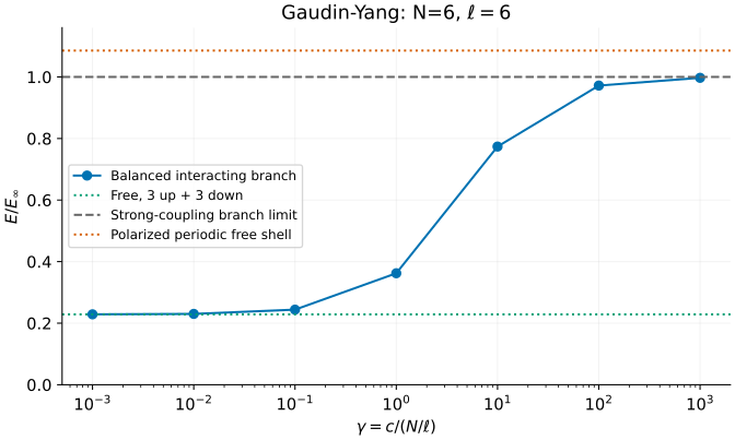
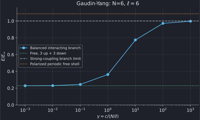
The balanced Gaudin–Yang energy rises from its free limit toward the interacting strong-coupling limit, below the distinct polarized periodic shell.

The normalization is the finite-N strong-coupling limit of this branch,

\[ E_\infty=\frac{\pi^2N(N^2-1)}{3\ell^2} =\frac{35\pi^2}{18}\quad(N=\ell=6). \]

The balanced free energy is \(4\pi^2/9\simeq4.38649084\). At small c,

\[ E-E_{\mathrm{free}}=\frac{2cN_\uparrow N_\downarrow}{\ell}+O(c^2)=3c+O(c^2). \]

At c=0.001 the exported shift is about 0.00299950; at c=1000 the energy is 19.13596659, approaching \(E_\infty\simeq19.19089745\) from below. The connecting line is a guide through finite calculations, not a thermodynamic interpolation.

The orange line is an independently exported fully polarized six-particle state on the same ring. It is free at every c, but its even-particle periodic shell has energy \(19\pi^2/9\simeq20.83583151\). It is not equal to the interacting branch's strong-coupling limit. Calling both limits “spinless” without matching their finite-ring shell conventions would hide this difference. It becomes a finite-size issue rather than a different bulk energy density.

3. Read two families of roots¶

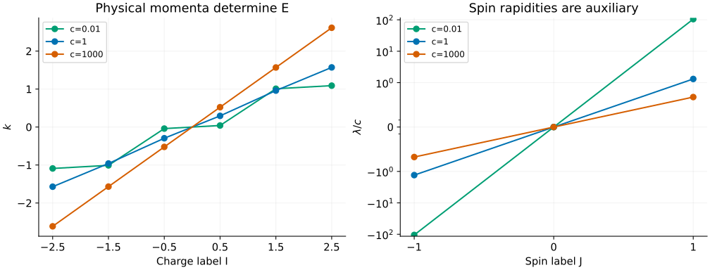
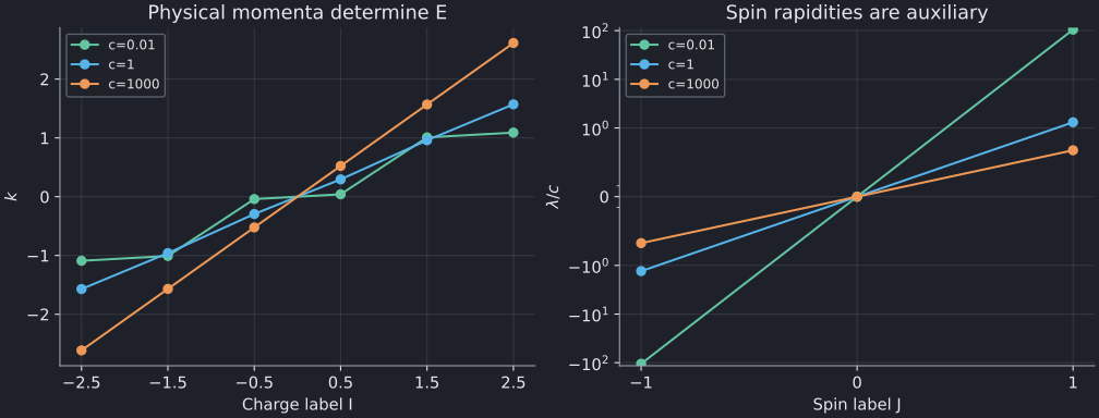
Charge momenta and spin rapidities at three couplings, plotted against their distinct Bethe labels.

The six charge roots are physical momenta k; their squares sum to E. The three spin roots are auxiliary rapidities, not additional particles whose squares should be included in the energy. Their natural strong-coupling scale grows with c, so the right panel plots \(\lambda/c\). Its vertical scale is symmetric-logarithmic (linear near zero), so the weak- and strong-coupling values can both be distinguished.

The two sets of labels are different: I are half-odd integers and J are integers for this centered branch. Joining rows merely by their array index would conflate distinct root families. The script checks both their labels and the original rational Bethe equations, not just the reported residual.

Physical momentum is \(P=\sum_j k_j\). It is not reduced modulo \(2\pi\): this is a continuum ring, with no lattice Brillouin zone. On a free branch, the frontend instead exports occupied integer modes. For example, N=4, two particles of each spin, c=0 and \(\ell=1\) selects modes 0 and 1 for each spin, giving P=\(4\pi\). Reflected choices have the same energy; the positive-current shell is a convention, not a unique free ground state.

4. Which calculations are supported?¶

The interacting centered branch requires both spin populations odd. Our 3+3 example satisfies this; 2+2 at c>0 does not. The rejected population is physically meaningful, but its periodic shell is not implemented. Do not change spin or labels silently to make a requested benchmark run.

Exact c=0 and fully polarized states are exceptions and allow arbitrary populations. Spin reversal is supported; the 5+3 and 3+5 saved examples have equal energies while keeping their physical population labels distinct.

The frontend does not yet compute attractive interactions, excitation lines, hard walls or thermodynamic integral equations. These are fixed-population ground-state benchmarks for finite systems, not spinon or holon dispersions.

Two particularly useful normalization checks are included:

Two opposite-spin particles at \(\ell=1,c=\pi\) obey the independent contact condition \(q\tan(q/2)=c/2\). The positive root is \(q=\pi/2\), giving \(E=\pi^2/2\).
Doubling the circumference and halving c preserves \(\gamma\) at fixed N. All physical roots halve and the energy becomes one quarter. The saved \(\ell=12,c=0.5\) example checks this against \(\ell=6,c=1\).

For a lattice MPS approximation to this continuum theory, match physical length, density, kinetic normalization and the coefficient 2c before comparing energies. Lattice-spacing errors are separate from root convergence. The model guide describes a controlled dilute-Hubbard comparison; a finite Hubbard ring is not literally the same Hamiltonian.

5. Reproduce and validate¶

The interacting scan's paired root tables and state exports are available here:

c	State	Charge roots	Spin roots
0.001	CSV	CSV	CSV
0.01	CSV	CSV	CSV
0.1	CSV	CSV	CSV
1	CSV	CSV	CSV
10	CSV	CSV	CSV
100	CSV	CSV	CSV
1000	CSV	CSV	CSV

The exact free c=0 path has a state and separate up / down occupations. Likewise, the polarized reference has a state, up occupations and an empty down table. These are deliberately not interacting charge/spin tables.

Additional check	State	Charge roots	Spin roots
Rescaled units	CSV	CSV	CSV
5 up + 3 down	CSV	CSV	CSV
3 up + 5 down	CSV	CSV	CSV
Two-body contact	CSV	CSV	CSV

The free-current example has state, up and down exports. All files retain invocation, precision, build provenance and status.

With the plotting dependencies installed, from the source checkout:

python3 scripts/plot_fermion_tutorial.py --check
python3 scripts/plot_fermion_tutorial.py
# Optional: regenerate the Gaudin–Yang and t–J examples together.
python3 scripts/plot_fermion_tutorial.py --solver-dir /path/to/bethe/bin
python3 -m unittest discover -s scripts -p 'test_tutorial_fermion.py'

The script validates root counts, equations, energy reconstruction, physical momentum and completed continuation at the requested c. Its tests add the contact oracle, weak/strong limits, unit scaling and corrupted exports. A residual tolerance is not an energy-error bound; failed continuation can leave an estimate that must not be used as a converged state. Examples use fp64, with native long-double and optional MPLAPACK fp128 available in the CLI.