Negative biquadratic chain: sectors, singlets and missing roots¶

View this page on GitHub

The free-end spin-1 chain with a negative pure biquadratic interaction is a useful test of symmetry-resolved MPS excitations. Its Bethe calculation uses an auxiliary spin-1/2 problem, but the physical multiplicities belong to a spin-1 chain. This tutorial makes that distinction concrete on four sites, then follows a complex-root singlet to longer chains.

The opposite-sign tutorial focuses on positive- energy defects above the ferromagnetic ground manifold.

1. Keep the sign and constant explicit¶

The default frontend Hamiltonian is

\[ H_-=-\sum_{i=1}^{N-1}(\mathbf S_i\cdot\mathbf S_{i+1})^2, \qquad S=1. \]

There is no bilinear term, added constant or physical boundary field. This is neither the ULS nor the Takhtajan–Babujian Hamiltonian. A single bond has energies −4, −1 and −1 in total spin 0, 1 and 2.

bethe-biquadratic-obc 2
bethe-biquadratic-obc 4

The ground energies should be \(-4\) and \(-(15+\sqrt{17})/2\), respectively. The default ground-state and sector helpers require even N with free ends. Do not infer an odd-chain or periodic-chain result from these commands.

2. Through-lines are not total spin¶

Define the nearest-neighbour singlet projector through

\[ e_i=(\mathbf S_i\cdot\mathbf S_{i+1})^2-1=3P_{0,i,i+1}. \]

These operators generate a Temperley–Lieb (TL) algebra. Its sectors, or modules, are labelled by a number of through-lines \(\ell\): unpaired strands in a diagrammatic basis. With \(M\) singlet arcs, \(N=\ell+2M\). This is algebraic bookkeeping, not a count of fixed singlet bonds in an eigenstate, and \(\ell/2\) is not the physical total spin.

One eigenvector of a TL module can occur many times in the physical spin-1 Hilbert space. On four sites:

Through-lines ell	TL eigenvectors	Physical states per eigenvector	Contribution to the Hilbert space
0	2	1	2
2	3	8	24
4	1	55	55

The sum is \(2+24+55=81=3^4\). In the ell=2 module, those eight physical states are one triplet plus one quintet. They are not eight spin multiplets or one multiplet of spin ell/2.

--spin-content resolves this multiplicity space into physical SU(2) multiplets. Its multiplets column counts irreducible multiplets; its magnetic_states column includes all \(2S+1\) projections. Join that table to the level table by state_id.

3. Find the singlet that real roots miss¶

Compare two requests in the same ell=0 module:

bethe-biquadratic-obc 4 --through-lines 0 --excitations all
bethe-biquadratic-obc 4 --through-lines 0 --q-spectrum --spin-content

The first returns only the ground configuration. The second uses a numerical Q-system search and finds both singlets, including the complex-root level:

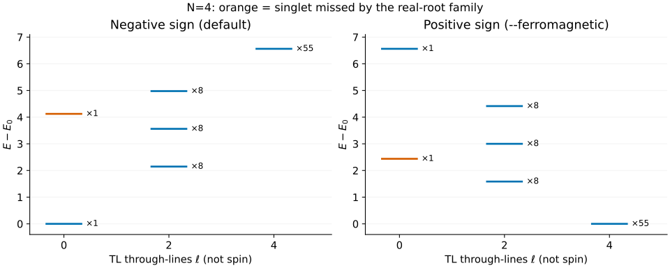
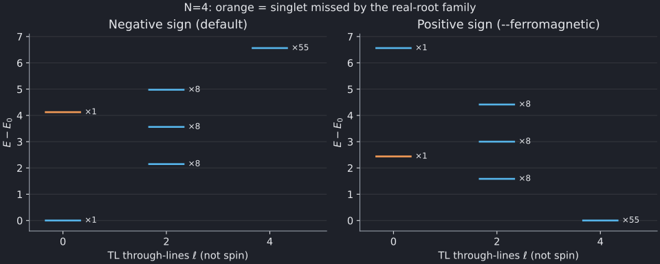
\[ E_{\pm}=\frac{-15\pm\sqrt{17}}2, \qquad E_+-E_-=\sqrt{17}. \]

Four-site gaps grouped by TL module for both Hamiltonian signs

The left panel is the default negative sign. Orange marks the singlet absent from the real-root scan; each annotation gives the number of physical states per TL eigenvector. The ell=2 levels lie at \(-6-\sqrt2,-6,-6+\sqrt2\), each eightfold. Some of these excitations lie below the excited singlet, so “singlet excitation” is not “first excitation of any spin”.

Download the Q-system results and spin decompositions:

Module	Levels	Spin content
ell=0	CSV	CSV
ell=2	CSV	CSV
ell=4	CSV	CSV

The real-root ell=0 export supplies the comparison. The tests check all four-site energies against the closed forms, all 81 states, and the full physical-spin count. Ground references computed by different numerical routes can leave a tiny roundoff offset from zero in the ground row's gap.

What does a successful Q-system search establish?¶

--q-spectrum searches one module. It reports the expected module dimension and number of discovered levels. A count match is a numerical completeness check, not a general mathematical certificate. An incomplete search returns discoveries that are not necessarily the lowest levels, even if they have been sorted by energy.

The four-site example has independent closed-form checks. Larger searches need more care; the frontend's spectrum regression coverage extends through N=8. Increasing --max-attempts helps discovery, while higher precision can help resolve roots. Neither replaces checking the final status.

4. Follow a selected singlet without enumerating the spectrum¶

For longer chains, use the targeted two-string solver:

bethe-biquadratic-obc 64 --singlet-excitation
bethe-biquadratic-obc 64 --singlet-excitation \
  --csv-table states=singlet.csv --csv-table reference=ground.csv

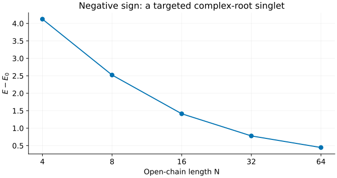
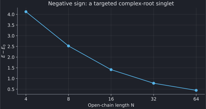
Finite-size gaps of the targeted negative-sign singlet

This selects a positive-deviation two-string above a real-root sea in ell=0. Its multiplicity is one physical singlet. It reproduces the excited four-site singlet and continues a selected branch; it does not search every state or certify the global first excited level on long chains.

N	Selected singlet	Global ground reference
4	CSV	CSV
8	CSV	CSV
16	CSV	CSV
32	CSV	CSV
64	CSV	CSV

The gap decreases substantially over these sizes. That trend alone is not evidence for a gapless thermodynamic limit. Match N and boundary conditions before judging an MPS error, and treat finite-size extrapolation separately from arithmetic precision or root-solver convergence.

5. Compare physical, not auxiliary, quantum numbers¶

The auxiliary XXZ model has anisotropy \(\Delta=3/2\) and opposite end fields. Its energy is converted by

\[ E_-=2E_{\mathrm{ref}}-\frac{7(N-1)}4. \]

Those fields are part of the auxiliary representation, not fields applied to the physical spin-1 chain. Running the ordinary zero-end-field bethe-xxz-obc at Delta=1.5 and shifting its energy is not equivalent.

For a finite MPS, use the physical energy, gap and spin_content, with the same free ends. There is no translation momentum. The finite even-chain ground state is a single singlet: do not attach a factor of two merely because the bulk phase is dimerized. Energies and spin multiplicities alone do not specify spectral weights for an operator.

6. Reproduce both sign tutorials¶

With the optional plotting environment:

python3 scripts/plot_biquadratic_tutorial.py
python3 scripts/plot_biquadratic_tutorial.py \
  --solver bethe-biquadratic-obc
python3 scripts/plot_biquadratic_tutorial.py --check
python3 -m unittest discover -s scripts -p 'test_tutorial_biquadratic.py'

The shared script regenerates both signs, validates every export before saving, and plots the numerical tables. These examples use fp64; native long-double and fp128 are available where supported.