ASEP: reduce the bias without changing the clock
All tutorials · Model guide · TASEP tutorial
ASEP allows both right and left hops on a periodic ring, still only into empty neighbouring sites. What happens to a relaxation mode when the hopping becomes symmetric? We will scan the bias on a 16-site, four-particle ring while keeping the sum of hopping rates fixed.
The TASEP tutorial introduces the generator convention. Here too the selected eigenvalue is \(\lambda=-g+i\omega\), with positive decay gap g and nonnegative angular frequency. These are inverse-time rates, not quantum energies.
1. Choose a meaningful path through the rates
Write the right/left rates as
We set R=1 and vary b from 1 (right-only TASEP) to 0 (symmetric exclusion). This avoids changing the basic timescale at the same time as the bias. The frontend accepts r and s directly; they need not sum to one.
# b=1/2, with r+s=1:
bethe-asep-pbc 16 --particles 4 --right-rate 0.75 --left-rate 0.25 \
  --csv-table relaxation=asep-mode.csv --csv-table roots=asep-roots.csv
The result is approximately
At b=1, the mode exactly matches the corresponding TASEP export. There is no independently chosen reference energy to subtract: the stationary eigenvalue is already zero.
2. Follow decay and oscillation separately
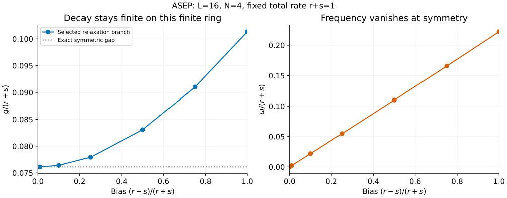
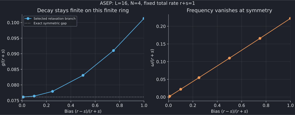
On this finite ring, the gap decreases toward a nonzero symmetric value while the frequency tends to zero. Consequently the long-time oscillation disappears, but relaxation remains. The graph does not establish a phase transition or a thermodynamic exponent: L is fixed, and connecting lines only guide the eye through the seven calculated biases.
At the symmetric endpoint r=s, every nontrivial filling has the exact gap
For L=16, R=1 this is approximately 0.07612046749. Separate half-filled and quarter-filled exports agree. As L grows this symmetric gap scales as \(L^{-2}\). The asymmetric fixed-density scaling in the TASEP tutorial is different; a fixed-L bias scan alone is not a controlled study of the large-L, weak-bias crossover.
There is also a useful analytic one-particle or one-hole result:
Its real part depends only on the total rate, while its frequency depends on the bias. Do not apply that one-particle formula to the interacting N=4 curve away from symmetry; the latter comes from Bethe roots and continuation.
3. What is being continued?
The solver starts with the finite-size TASEP relaxation branch and follows it to the requested ratio \(x=\min(r,s)/\max(r,s)\). The equations and eigenvalue conventions follow Golinelli–Mallick's ASEP review, Eqs. (66) and (69). Full small-ring spectra independently check the branch selection, but continuation is not an exhaustive proof that no other branch overtakes it at every size and rate.
Near symmetric hopping, ordinary Bethe coordinates crowd near one. The exported roots instead use finite scaled coordinates:
Metadata supplies the wave-root index and the complex wave base \(w=e^{\pm2\pi i/L}-1\). The roots table contains v, not z or momenta. The tutorial script reconstructs z to check the eigenvalue and multiplicative Bethe equations. This reconstruction is adequate for these examples, whose smallest nonzero bias is 0.01; it is not a substitute for the native solver's scaled arithmetic at biases close to machine precision.
At exactly symmetric hopping, and in the one-particle/one-hole cases, the result is analytic and the roots table has no rows. That is an intentional representation, not a failed export. Empty/full sectors likewise succeed but have no nonstationary mode: their gap and frequency are absent.
The default arithmetic is fp64; native long-double, configured fp128 and explicit MPFR/MPC are supported. The saved examples retain their original arithmetic. A converged residual is a numerical diagnostic, not a rigorous error certificate. Failed continuation cannot be accepted at the last reached ratio: the frontend exits with failure and leaves physical observables missing.
4. Symmetries and non-Hermitian comparisons
Multiplying both rates by two doubles the whole generator spectrum. Swapping r and s reflects the ring; particle–hole symmetry maps N to L-N. All three operations are checked in the saved examples. Reflection and particle–hole symmetry preserve the reported nonnegative-frequency representative, not the propagation direction of a fixed momentum-labelled mode.
For a matrix-product calculation, match the ring boundary, population, total rate and bias. Compare both parts of the complex eigenvalue; comparing only its magnitude confounds oscillation with decay. If working with -M instead, reverse the eigenvalue sign. The supplied energy-like numbers do not provide biorthogonal matrix elements, mode amplitudes or the overlap of an observable with the slow mode.
Open reservoirs are another problem: they change the stationary state, boundary conditions and spectral structure. Neither periodic frontend accepts reservoir rates or enumerates a full spectrum.
5. Reproduce and validate
The fixed-total-rate scan is available as paired exports:
| b | r | s | Relaxation mode | Scaled roots |
|---|---|---|---|---|
| 1 | 1 | 0 | CSV | CSV |
| 0.75 | 0.875 | 0.125 | CSV | CSV |
| 0.5 | 0.75 | 0.25 | CSV | CSV |
| 0.25 | 0.625 | 0.375 | CSV | CSV |
| 0.1 | 0.55 | 0.45 | CSV | CSV |
| 0.01 | 0.505 | 0.495 | CSV | CSV |
| 0 | 0.5 | 0.5 | CSV | empty CSV |
Additional checks use the same provenance/status format:
| Check | Mode | Roots |
|---|---|---|
| Double both rates | CSV | CSV |
| Reflect the rates | CSV | CSV |
| Particle–hole, N=12 | CSV | CSV |
| One particle | CSV | empty CSV |
| Symmetric half filling | CSV | empty CSV |
| Empty ring | CSV | empty CSV |
| Full ring | CSV | empty CSV |
| L=5, N=2, r=1, s=1/2 | CSV | CSV |
From the source checkout, with the plotting dependencies:
python3 scripts/plot_exclusion_tutorial.py --check
python3 scripts/plot_exclusion_tutorial.py
# Optional: regenerate the TASEP and ASEP examples together.
python3 scripts/plot_exclusion_tutorial.py --solver-dir /path/to/bethe/bin
python3 -m unittest discover -s scripts -p 'test_tutorial_exclusion.py'
The shared script reads native exports for each point, joins mode/root tables by provenance, and rejects failed, missing or inconsistent observables. The tests also verify a separate ten-configuration generator at L=5, N=2, the analytic endpoints and all the symmetries above. The horizontal symmetric-gap guide is explicitly analytic; the plotted bias scan is not an interpolation of endpoint formulas.