Central spin: sector energies and field response
All tutorials · Model guide · Richardson tutorial
One spin coupled to an inhomogeneous bath makes a useful long-range MPS benchmark. Here we compare fixed-magnetization ground energies, verify the zero-field multiplet and infer a central-spin response from energy differences. The solver supplies energies and regular Gaudin variables, not time evolution or wavefunctions.
1. Specify the star, not a spatial chain
Our Hamiltonian is
Every spin is 1/2. B acts only on the central spin; there are no bath fields or bath–bath couplings. The positive sign of B means a large positive field favours a down central spin. The Gaudin conventions follow Faribault–Schuricht, with bath field zero. Their dynamical calculations require capabilities beyond this ground-energy frontend.
Choose three bath couplings 1,0.7,0.3, central field 1 and total Sz=0:
bethe-central-spin --couplings 1,0.7,0.3 --field 1 --sz 0 \
  --csv-table states=central-state.csv --csv-table variables=central-variables.csv
The energy is approximately -1.11248592. --sz includes the central spin,
so four total spins allow sectors -2,-1,0,1,2. A sector minimum is not
automatically the global minimum. Repeating this command with --sz 1 gives
-1.22153504, already lower at this field.
Couplings can have either sign, but must be nonzero and distinct. Input order is preserved for reporting and does not change the energy. Repeated couplings and decoupled zero-coupling bath spins require different sector bookkeeping; do not approximate them by silent perturbations.
2. Compare sectors across field
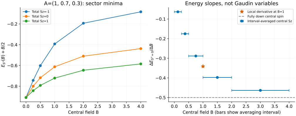
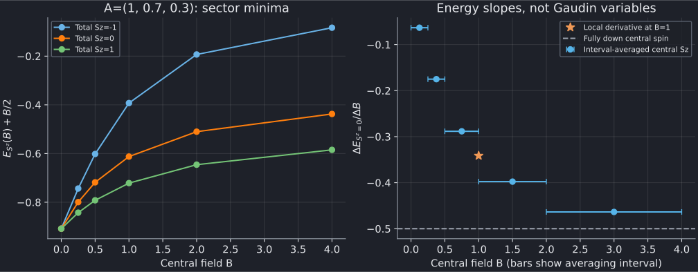
The left panel plots E+B/2 to remove the leading central-down Zeeman term visually. The CSV files contain the absolute Hamiltonian energy E; this display shift is not an extra term in the Hamiltonian and must be removed before differentiating the plotted quantity.
At B=0, the Sz=-1,0,+1 minima agree at approximately -0.90870128. They are components of a zero-field SU(2) multiplet, not evidence that an Sz=0 calculation found a singlet. A finite central-only field splits them. The completely polarized sectors provide a separate exact check:
Do not assume that a fixed-sector energy decreases from B=0: the Sz=-1 branch initially increases, before bending down. The relevant general check is concavity of the lowest energy in each fixed sector, since H depends linearly on B. Energies from different sectors should not be spliced together when estimating that sector's response.
Spin reversal gives another useful identity:
The downloads verify it at B=±1, as well as coupling permutation and a common factor-two scaling of all A and B. These are normalization checks, not a claim that the central spin and bath spins are interchangeable.
3. Estimate central polarization from energies
For a normalized, nondegenerate eigenstate in a fixed sector, the Hellmann–Feynman relation reads
The right panel uses the unshifted Sz=0 energies. Each blue marker is a secant slope, with a horizontal bar spanning the two sampled fields:
It is an interval average, not the exact magnetization at the midpoint. The bars are averaging intervals, not statistical error bars. Their values lie between -1/2 and +1/2 and decrease with field, consistently with concavity.
To obtain a local estimate at B=1, the starred point uses centered differences:
| Field step h | \([E(1+h)-E(1-h)]/(2h)\) |
|---|---|
| 0.01 | -0.34140475 |
| 0.005 | -0.34140757 |
The difference is about \(2.8\times10^{-6}\). The refined estimate agrees within \(2\times10^{-6}\) with a direct small-matrix expectation value in the optional validation. Neither agreement nor the solver residual is a rigorous derivative error bar. Smaller h reduces finite-difference truncation but eventually amplifies energy roundoff; test h and precision together.
At large positive field the central spin approaches -1/2. The extra B=100 run checks the high-field product-state energy for this sector, with the two largest bath couplings carrying up spins. With mixed-sign couplings, “largest” means algebraically largest, not largest absolute value.
4. Gaudin variables are not magnetizations
The implementation uses the quadratic-variable strategy of Faribault et al., also used in the pairing tutorial. The physical Hamiltonian and state-selection seed are different; selecting a Richardson ground state is not a shortcut to selecting this central-spin ground state.
For the B=1, Sz=0 example the central variable is approximately -0.74165728, and the first bath variable is approximately 1.00008328. Neither is a spin projection or occupation probability. The central polarization from the energy derivative is instead approximately -0.341408.
At B=0 the solver evaluates the exact zero-field equations, not a tiny-field substitute. The compactified variables stay finite and sum to zero there; that does not say there are no up spins. At negative B they describe the spin-reversed computational frame. The reported physical field and total Sz retain their requested signs.
For analytic polarized or isolated-spin cases, variable entries are missing
because no continuation variables are needed. A missing variable is not zero.
On incomplete continuation an energy, if present, belongs to reached_field,
not necessarily requested_field; the initial infinite-field seed has no
finite reached field or energy at all. Reject those runs before plotting a
target-field curve.
For MPS comparisons use the same star Hamiltonian and total-Sz sector. Mapping the bath to an MPS ordering changes the representation, not the couplings. There is no lattice momentum, PBC/OBC switch or homogeneous iMPS dispersion here. Excitation spectra, form factors, bath dynamics and higher local spins are not implemented in this frontend.
5. Reproduce and validate
Native field-scan exports (each cell links the state and regular variables):
| B | Total Sz=-1 | Total Sz=0 | Total Sz=+1 |
|---|---|---|---|
| 0 | state / variables | state / variables | state / variables |
| 0.25 | state / variables | state / variables | state / variables |
| 0.5 | state / variables | state / variables | state / variables |
| 1 | state / variables | state / variables | state / variables |
| 2 | state / variables | state / variables | state / variables |
| 4 | state / variables | state / variables | state / variables |
| Derivative run | State | Variables |
|---|---|---|
| B=0.99 | CSV | CSV |
| B=1.01 | CSV | CSV |
| B=0.995 | CSV | CSV |
| B=1.005 | CSV | CSV |
| Additional check | State | Variables |
|---|---|---|
| One bath spin, A=B=1 | CSV | CSV |
| One bath spin, B=0 | CSV | CSV |
| Spin-reversed field/sector | CSV | CSV |
| Permuted bath inputs | CSV | CSV |
| All energy scales doubled | CSV | CSV |
| Polarized up | CSV | nulls |
| Polarized down | CSV | nulls |
| Isolated spin | CSV | null |
| Mixed-sign bath, B=0 | CSV | CSV |
| Mixed-sign bath, B=2 | CSV | CSV |
| High field B=100 | CSV | CSV |
With the plotting dependencies, from the source checkout:
python3 scripts/plot_gaudin_tutorial.py --check
python3 scripts/plot_gaudin_tutorial.py
# Optional: regenerate this and the Richardson tutorial.
python3 scripts/plot_gaudin_tutorial.py --solver-dir /path/to/bethe/bin
# Optional independent matrices and central-polarization check; requires NumPy.
python3 scripts/plot_gaudin_tutorial.py --check --oracle
python3 -m unittest discover -s scripts -p 'test_tutorial_gaudin.py'
The script checks every quadratic equation, number constraint, input/variable join and energy reconstruction. Its optional oracle independently builds and diagonalizes each saved spin sector; no Bethe equations enter those matrices. The tests also cover the exact two-spin energy, analytic null variables, zero-field degeneracy, reversal, scaling, concavity and rejection of incomplete or corrupted outputs. Native long-double and optional MPLAPACK fp128 provide precision controls without changing the model.