Bose–Fermi mixtures: change statistics, not just a component label¶

All tutorials · Model guide · SU(n) fermion tutorial

This gas contains scalar bosons and spinless fermions of equal mass. Boson–boson and boson–fermion contact strengths are equal; identical fermions do not feel the contact interaction. It is a graded integrable model, not another color of the multicomponent Fermi gas.

We will hold total particle number and circumference fixed, vary the repulsion, and then compare selected compositions. The outputs are finite-ring ground states, not excitation dispersions or correlation functions.

1. Fix the equal-coupling Hamiltonian¶

The first-quantized convention is

\[ H=-\sum_j\partial_{x_j}^2+2c\sum_{i\lt j}\delta(x_i-x_j),\qquad \frac{\hbar^2}{2m}=1,\qquad c\ge0. \]

Particle statistics determine which contact terms survive. Changing either mass or the ratio of boson–boson to boson–fermion couplings leaves the model implemented here. The equations follow Imambekov–Demler, Eqs. (3), (28)–(34).

Choose two bosons and three fermions on a circumference-five ring:

bethe-bose-fermi-pbc --bosons 2 --fermions 3 --length 5 --c 1 \
  --csv-table states=bf-state.csv --csv-table charge_roots=bf-charge.csv \
  --csv-table auxiliary_roots=bf-auxiliary.csv

The total density is one, energy is approximately 5.47425839, and momentum is zero. Length is a physical circumference, not five lattice sites.

2. Sweep repulsion, then compare compositions¶

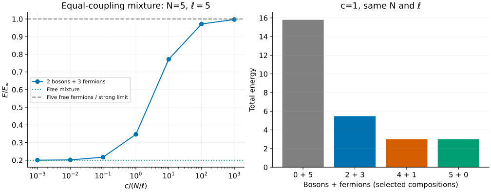
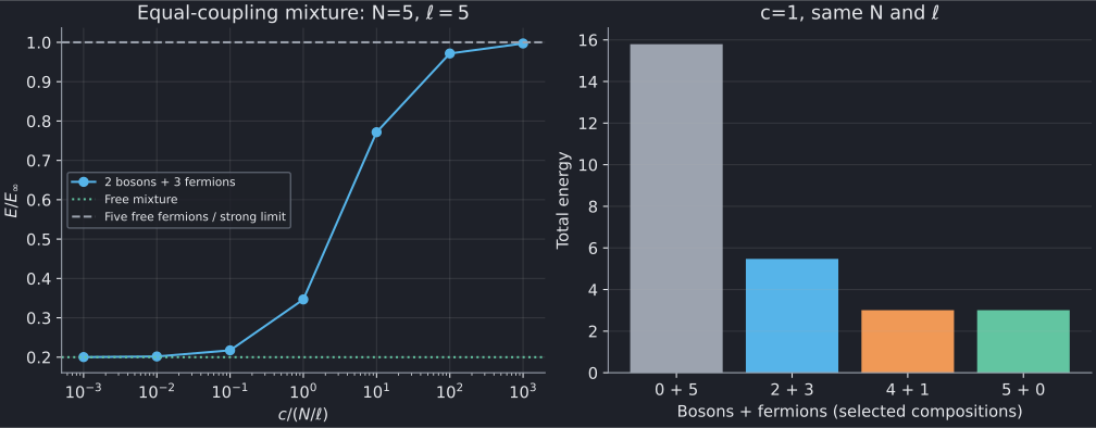
A two-boson three-fermion energy rises with repulsion; composition benchmarks at c=1 show the pure-boson and one-fermion energies coincide.

The left panel divides by the finite-size impenetrable limit

\[ E_\infty=\frac{\pi^2N(N^2-1)}{3\ell^2} =\frac{8\pi^2}{5}\quad(N=\ell=5). \]

This also equals the energy of five free spinless fermions on this odd-particle ring. The c=0 mixture instead has all bosons at k=0 and fermions in integer modes -1,0,1, giving E approximately 3.15827341. Its initial slope is

\[ E-E_{\mathrm{free}}= \frac{cN_b(N_b-1)+2cN_bN_f}{\ell}+O(c^2)=\frac{14}{5}c+O(c^2). \]

The first term counts boson–boson contacts and the second boson–fermion contacts. At c=0.001 the shift is about 0.00279940. At c=1000 the energy is 15.74575939, approaching the strong-coupling reference 15.79136704. Markers are native solutions; connecting lines do not replace a thermodynamic calculation.

The right panel changes the composition at fixed N=5, circumference 5 and c=1. Five fermions have no interacting contacts, whereas five bosons have the Lieb–Liniger energy 3.00678253. Four bosons plus one fermion have the same spatial ground energy: one fermion introduces no exchange antisymmetry between identical fermions. The native mixture and separate Lieb–Liniger exports agree in their charge roots as well as energy.

This equality does not identify species-resolved observables or correlation functions. Nor does a four-bar finite-size comparison establish a demixing phase diagram. Only energies of the displayed supported compositions are shown.

3. The auxiliary roots count bosons¶

The mixed branch has N charge momenta and N_b auxiliary rapidities:

\[ \begin{aligned} \ell k_j+\sum_a2\arctan\frac{2(k_j-\lambda_a)}c&=2\pi I_j,\\{} \sum_j2\arctan\frac{2(\lambda_a-k_j)}c&=2\pi J_a,\\{} E&=\sum_j k_j^2. \end{aligned} \]

Our two-boson, three-fermion example therefore exports five charge roots and two auxiliaries. There is no auxiliary–auxiliary scattering term, unlike the spin equations of an SU(n) Fermi gas. The labels J use the sign convention in our guide; they are opposite to the paper's auxiliary logarithmic labels. Only charge momenta contribute directly to the energy.

The pure-boson path delegates to Lieb–Liniger and has an empty auxiliary table. At c=0, or with no bosons, the frontend instead returns species-labelled free occupations. Repeated boson k=0 rows are valid occupations, not accidentally duplicated interacting roots.

4. Shell restrictions and useful benchmarks¶

With c>0 and both species present, the centered periodic branch requires odd N_f; N_b may be odd or even. That is why the composition plot shows 0+5, 2+3, 4+1 and 5+0, but not 1+4 or 3+2. Those omitted mixtures are physical states whose shells are not implemented. Pure species, vacuum and c=0 accept arbitrary counts.

Free even-fermion shells choose the positive-current representative. The saved c=0 example with two bosons, two fermions and circumference 1 has boson modes 0,0 and fermion modes 0,1. Its momentum is \(2\pi\), not zero: continuum momentum is not folded modulo \(2\pi\).

Further checks make the numerical conventions explicit:

One boson plus one fermion at circumference 1 and c=\(\pi\) has \(E=\pi^2/2\), from the two-body contact condition.
Doubling circumference and halving c keeps the dimensionless interaction fixed: physical roots halve and energy is divided by four.
Pure bosons and the one-fermion example agree with a separately run Lieb–Liniger frontend at the same N, circumference and c.

For a continuum MPS discretization, match species statistics, masses and both interaction coefficients before comparing energies. Bosonic occupation truncation and lattice spacing are additional approximation controls; the Bethe residual does not measure either error. Excitations, unequal couplings, attraction, traps and open boundaries are outside this frontend's scope.

5. Reproduce and validate¶

c, N_b=2 and N_f=3	State	Charge roots	Auxiliary roots
0.001	CSV	CSV	CSV
0.01	CSV	CSV	CSV
0.1	CSV	CSV	CSV
1	CSV	CSV	CSV
10	CSV	CSV	CSV
100	CSV	CSV	CSV
1000	CSV	CSV	CSV

Other interacting case	State	Charge roots	Auxiliary roots
Five bosons	CSV	CSV	empty CSV
Four bosons, one fermion	CSV	CSV	CSV
Rescaled 2+3	CSV	CSV	CSV
Two-body contact	CSV	CSV	CSV

Free cases have different tables:

Case	State	Species-labelled occupations
c=0, 2+3	CSV	CSV
Five fermions	CSV	CSV
Free even shell	CSV	CSV
Vacuum	CSV	empty CSV

The independent Lieb–Liniger run supplies a state and roots. All exports retain provenance and status.

With the plotting dependencies, from the source checkout:

python3 scripts/plot_multicomponent_tutorial.py --check
python3 scripts/plot_multicomponent_tutorial.py
# Optional: regenerate this and the SU(n) tutorial, including reference runs.
python3 scripts/plot_multicomponent_tutorial.py --solver-dir /path/to/bethe/bin
python3 -m unittest discover -s scripts -p 'test_tutorial_multicomponent.py'

The script validates species, root counts, labels, equations, energy and unwrapped momentum. Its tests check model reductions, weak/strong limits, units, free shells and corrupted exports. Failed solves must be rejected, not plotted as zero energy. These examples use native fp64; long-double and optional MPLAPACK fp128 use the same equations and sector rules.