Comparing two-, four- and six-spinon spectra
Four-spinon refinement · Six-spinon sampling · Selected-sector calculations · Direct moments
An energy continuum tells us where an excitation can occur. A dynamical structure factor also measures how strongly the chosen spin operator excites it. Here we compare contributions to the longitudinal response of the infinite spin-\(1/2\) Heisenberg chain,
at zero temperature and field. We use \(q=\pi/2\), frequencies in units of \(J\), and the unbroadened density \(S^{zz}(q,\omega)\). Its frequency moments use \(d\omega/(2\pi)\). Bethe supplies the physical normalization of every sector; no plotting multiplier or adjustment to a sum rule is needed.
Choose a learning or reference workflow
For a hands-on calculation, start with the two-spinon density, small four-spinon example, or six-spinon sampling examples. These introduce the commands, normalization and diagnostics at modest cost. The small four- and six-spinon examples use restricted integration domains; they are not converged replacements for the reference spectra.
This comparison uses large-domain reference calculations. The checked compact record can be redrawn using only the plotting tools; no integrations are run. Regenerating the reference is a separate, optional production task. Consult the two/four-spinon compute budget and six-spinon compute budget before running those recipes. Their settings and costs describe the saved datasets; benchmark a representative complete query before budgeting new work.
Read the reference comparison
The sixteen requested frequencies now have checked two-, four- and six-spinon results. The left panel separates the three contributions; the right compares their partial sums on the same logarithmic density scale.
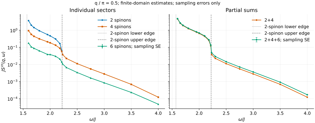
Above the two-spinon upper edge, the blue contribution is exactly zero. The four- and six-spinon contributions continue, so the difference between the \(2+4\) and \(2+4+6\) curves directly shows the extra six-spinon response. Inside the two-spinon band, compare the individual sectors as well as the sums: a smaller contribution can be difficult to see on a curve dominated by \(S^{zz}_2\).
Symbols mark calculated values; joining lines guide the eye. The plotted range ends at \(\omega/J=4\), before the outer four- and six-spinon edges. The bars on \(S^{zz}_6\) and \(S^{zz}_{2+4+6}\) are the same observed sampling standard error. Their relative size for the six-spinon contribution ranges from 2.49--6.52%; 15 of the sixteen points meet the initial 5% sampling target. They exclude the deterministic quadrature, contour, arithmetic and omitted-domain uncertainties discussed below, as well as uncertainty from rare configurations not adequately sampled.
Download the combined compact data, or use the fast redraw command. The validation record keeps each sector, its sampling diagnostics, the original source identities and the checks used to assemble the comparison. The original two/four data and the new six-spinon data come from different Bethe revisions; the reviewed source comparison explains why they can be joined without changing their recorded provenance.
What the comparison tests
At this momentum the two-spinon continuum lies between
Four and six spinons contribute inside this interval and above its upper edge. That higher-frequency signal is a useful test of spectral calculations: a two-spinon reference alone vanishes there even though the full spin response need not. Conversely, weight inside the two-spinon continuum need not come only from two spinons.
The quantities to compare are the individual \(S^{zz}_2\), \(S^{zz}_4\) and \(S^{zz}_6\), followed by the partial sums
Neither partial sum includes eight and higher sectors. A sector's fraction of the integrated sum rule is not its fraction at each frequency, so multiplying the two-spinon curve by a global weight ratio does not generate these sums.
The comparison uses a shared logarithmic density scale so the weaker individual sectors remain visible, including above the two-spinon upper edge. The dotted and dashed vertical lines mark the lower and upper two-spinon edges, respectively. A physical zero cannot appear on that scale: the two-spinon line stops at its last positive sample. The compact data retain the zeros and distinguish them from failed or unavailable values. Lines joining samples are visual guides, not interpolated data for further calculations. Nonzero values outside the plotting format's range are rejected explicitly rather than being displayed as zero. The horizontal range retains every requested frequency, even where all displayed values are zero or unavailable, together with the two edge guides. If six-spinon results are missing, the figure states how many requested frequencies are unavailable. Both six-inclusive curves retain those gaps; an entirely unavailable sector is labelled as such in the legend.
Checks behind the reference calculation
Before generating new reference data, start at a few interior frequencies on both sides of the two-spinon upper edge. Avoid an exactly singular threshold as a finite plotting sample. At each anchor, check the individual contributions before requesting a dense grid. These checks belong to reference generation; reading or redrawing an existing compact record does not repeat them.
- For four spinons, increase quadrature order at a fixed soft domain, then extend the domain at fixed order. The refinement tutorial shows why a small order difference alone is insufficient.
- For six spinons, inspect independent replicate means, sampling errors and influential observations. Compare proposal choices using independent validation samples after tuning. Separately extend the rapidity domain.
- Repeat representative calculations with stronger arithmetic and contour controls. Those comparisons test density evaluation; they do not recover configurations omitted by a finite domain or missed by sampling.
The four-spinon cutoff is a log-radius cutoff; the six-spinon cutoff bounds absolute rapidities. Equal cutoff numbers describe different integration domains. The final comparison needs a separate domain study for each sector. Sampling error bars should retain their statistical meaning; a cutoff change is a separate numerical comparison, not another sampling variance. The \(S^{zz}_{2+4+6}\) curve carries the same sampling standard error as \(S^{zz}_6\); the deterministic two- and four-spinon contributions do not add sampling variance. Their numerical and domain uncertainties remain separate.
Failed requested sectors remain absent, and their partial sum is incomplete. Do not interpolate across a failed point or replace it with zero. A successful finite-domain result still needs the convergence checks above before it is interpreted as an unrestricted physical response.
Use the same declared frequency grid for all sectors. Different arithmetic
formats can serialize an input such as 1.8 to slightly different binary
approximations. The data reader matches each computed coordinate uniquely
within its recorded rounding allowance, preserving both computed values
alongside the requested input. It rejects missing, colliding or ambiguous
nodes; this matching does not interpolate or move spectral weights between
distinct requested frequencies.
Measured four-spinon controls
The calibration record keeps the complete queries, effective controls, raw-export hashes and observed changes used to choose the display calculation. Below the two-spinon upper edge, extending the soft domain matters much more than increasing arithmetic precision. At \(\omega/J=2\), fixed order 4 gives \(S^{zz}_4=0.137056\) at log-radius cutoff 12 and \(0.183538\) at cutoff 768. The latter is about 34% larger. Tiny density diagnostics at the smaller cutoff cannot reveal those omitted configurations.
Refining the larger-domain calculations gives:
| \(\omega/J\) | Latest \(J S^{zz}_4\) | Fixed-domain order comparison | Relative change |
|---|---|---|---|
| 1.6 | 0.942545 | 4 to 8, cutoff 768 | +0.3145% |
| 2.0 | 0.184090 | 4 to 8, cutoff 768 | +0.3013% |
| 2.23 | 0.0378453 | 16 to 32, cutoff 24 | +0.01952% |
| 3.0 | 0.00278670 | 32 to 64, cutoff 24 | +0.4951% |
| 4.0 | 0.000121906 | 32 to 64, cutoff 24 | +0.4214% |
Domain comparisons remain separate. At order 8, extending cutoff 384 to 768 raises the results at \(\omega/J=1.7\) and \(2\) by 0.6973% and 0.5509%. Near the lower edge, the corresponding order-4 change at \(1.6\) is 0.8251%. Just above the upper edge, at \(2.23\), cutoffs 24 and 48 give identical exported values in the order-4 check. This last comparison is a coarse-order domain check; it is not a claim about every quadrature order or frequency. None of these observed differences bounds the remaining tail or total error.
The same above-edge frequency separates density controls from outer integration. At fixed order 16 and cutoff 24, increasing geometry from 192 to 256 bits and density comparisons from 128/192 to 192/256 bits changes the result by \(1.54\times10^{-57}\) relative. With the wider arithmetic held fixed, increasing residue budgets from 64/80 to 96/112 and tail orders from 16/20 to 24/28 changes it by \(6.43\times10^{-38}\). These checks explain why outer quadrature and domain refinement, rather than more density digits, control this comparison.
Geometry and density precision are separate controls. The saved deep-domain four-spinon calculation uses 1536-bit geometry with 192/256-bit density checks. At \(\omega/J=2\), cutoff 768 and order 4, the density comparison agrees with a 1472/1536-bit reference within \(7.90\times10^{-76}\) relative. This supports the density choice at that query; it does not measure the minimum geometry precision. Validate a different geometry setting on the four-spinon quadrature itself, including support and weighted contributions. The accuracy guide explains the procedure. The development study records the implementation and cost comparisons separately.
The optional reproduction recipe records the full display grid and controls. The much smaller four-spinon example is a quicker way to learn the commands.
Compare with time-evolution calculations
Match the Hamiltonian, operator normalization and Fourier conventions first.
The raising channel is twice the longitudinal channel at zero field; unit-cell
normalizations in an MPS calculation are a separate convention to check.
A finite time window introduces frequency resolution. Apply the same resolution kernel to an integrated reference when comparing frequency-domain curves; unbroadened threshold values cannot be compared directly to a finite-height broadened peak. Alternatively, Fourier transform the properly integrated spectral contributions to compare in the time domain.
Use direct moments for intensity or first-moment checks. Integrating the sparse display points, particularly near an edge, does not establish the sum rules or the omitted higher-sector weight.