XXZ spinons and two-spinon continua¶

View this page on GitHub

This tutorial produces reference curves for an infinite spin-1/2 XXZ chain, then shows how to compare them with an MPS excitation calculation. We compare the gapless Heisenberg point with a gapped antiferromagnet. No finite-size extrapolation is required.

You can read the plots immediately. To reproduce the data, build Bethe with bethe-xxz-dispersion; the default fp64 build suffices here. Python and Matplotlib are optional, used only to redraw the figures.

1. Fix the normalization¶

We use zero magnetic field, zero temperature, and exchange \(J=1\):

\[ H=J\sum_j\left(S_j^xS_{j+1}^x+S_j^yS_{j+1}^y+ \Delta S_j^zS_{j+1}^z\right),\qquad S^\alpha=\sigma^\alpha/2. \]

The plotted energies are excitation energies above the thermodynamic ground state, in units of J. They are not the ground-state energy per site reported in the command's overview. If your Hamiltonian uses Pauli matrices instead of spin operators, account for the factor of four before comparing energies.

The lattice spacing is one. The elementary spinon momentum is p; the two-spinon total constituent momentum is Q. Both are measured in radians per site, but their exported ranges differ.

2. Export the curves¶

Run in your chosen calculation directory, with the executables on PATH (or use ./bethe-xxz-dispersion from its build directory; see setup):

bethe-xxz-dispersion --delta 1 --points 401 --csv xxz-delta1.csv
bethe-xxz-dispersion --delta 2 --points 401 --csv xxz-delta2.csv

The default --branch all exports both families in the dispersion table. Each file contains 401 spinon rows and 401 two-spinon rows. Lines starting with # record the Hamiltonian, conventions, precision, source revisions, command, convergence and timing. Keep them with the data.

`branch`	Horizontal coordinate	Populated energy columns
`spinon`	`p_over_pi`, from 0 to 1	`energy`
`two-spinon`	`p_over_pi`, now Q/π, from 0 to 2	`lower`, `upper`

Empty energy cells in the other columns are intentional. Do not treat them as zeros. Check the process exit status, final success metadata and each row's status before plotting. For larger workflows, --csv-table dispersion=FILE selects this same table explicitly; see export options.

3. Read the spectrum¶

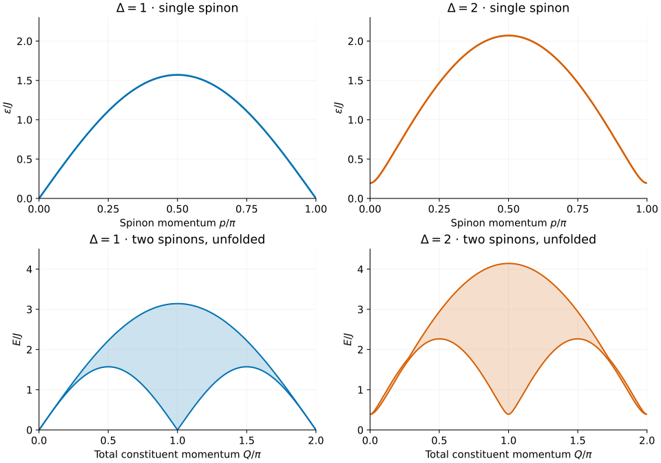
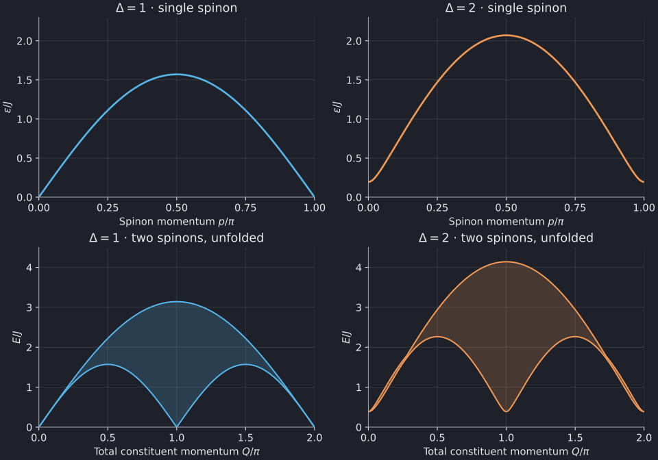
Single-spinon energies above unfolded two-spinon continuum bounds, with Delta 1 on the left and Delta 2 on the right. The Delta 2 spinon has a nonzero endpoint gap.

Full-size figure: light · dark.

At \(\Delta=1\), the elementary line is

\[ \epsilon(p)=\frac{\pi J}{2}\sin p,\qquad 0\le p\le\pi. \]

It is gapless at both endpoints and reaches \(\pi J/2\) in the middle. This is a useful first normalization check on both the exported data and an MPS result.

At \(\Delta=2\), the single-spinon gap is approximately 0.194901 J and the maximum energy is 2.070496 J. The minimum two-spinon energy is twice the single-spinon gap, approximately 0.389802 J. All curves in the figure come from the exported data, not a separate Python implementation of the formulas.

The shaded regions contain the energies obtained by adding two spinon energies at fixed total constituent momentum:

\[ E=\epsilon(p_1)+\epsilon(p_2),\qquad Q=p_1+p_2\pmod{2\pi},\qquad 0\le p_1,p_2\le\pi. \]

Shading means kinematic support, not spectral intensity. It does not show matrix elements, selection rules, or higher-particle continua. In particular, the unfolded constituent branch shown here should not be identified without qualification with the support of a particular dynamical structure factor.

4. Match a two-site MPS unit cell¶

For \(\Delta\gt1\), the two Néel vacua are related by translation by one site. A single spinon connects different vacua on its left and right. It belongs in a domain-wall (topological) excitation ansatz and carries \(S^z=\pm1/2\). A local excitation above one fixed vacuum has the same vacuum at both ends; the two-spinon sector, with \(S^z=-1,0,+1\), is a natural reference. These are spin-projection labels, not generic SU(2) total-spin labels.

Translation by a two-site unit cell measures only

\[ q_{\mathrm{cell}}=2p\pmod{2\pi} \]

(replace p with Q for a pair). Thus momenta separated by π are identified. The spinon interval already spans one cell Brillouin zone. For the pair, ask for the union with the π-shifted translation branch:

bethe-xxz-dispersion --delta 2 --points 401 --folded --csv xxz-delta2-folded.csv

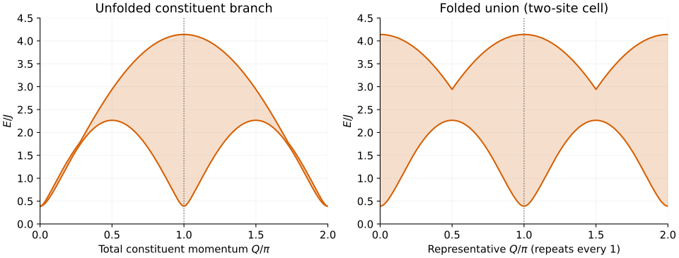
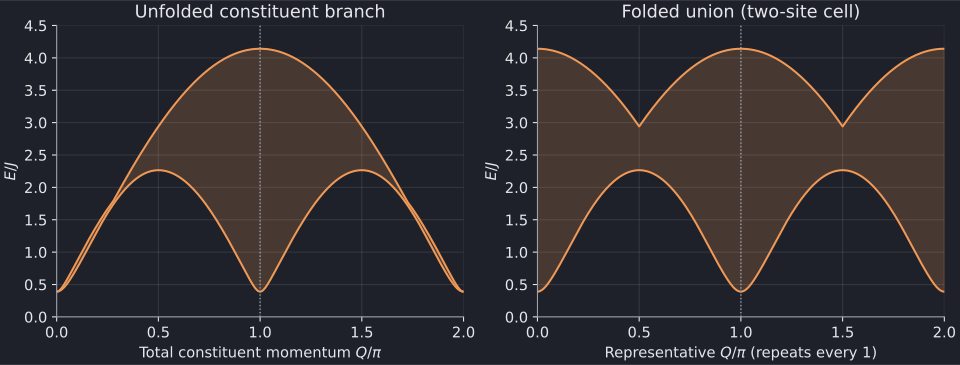
Delta 2 two-spinon continuum before and after folding. The folded union repeats with period pi and includes the broad continuum at both zero and pi.

Full-size folding comparison: light · dark.

The right panel still uses the exported representative Q/π on [0,2], so it shows two copies of the reduced zone. For an MPS plot against \(q_{\mathrm{cell}}/\pi\), take just \(0\le Q/\pi\lt1\) and multiply that horizontal coordinate by two. Do not sort all exported rows by cell_momentum and connect them: the repeated representatives can produce misleading lines.

Folding the energy envelope does not make an observable's spectral weight π-periodic. One-site translation sectors may carry different or vanishing matrix elements. In the gapless chain, the same operation is ordinary zone folding, not evidence for two symmetry-broken vacua.

Before comparing an MPS result, check:

Spin versus Pauli normalization and the exchange J.
Excitation energy versus bulk energy density.
Momentum in radians/site versus translation phase per unit cell.
Domain-wall versus same-vacuum excitation sector.
Continuum edges versus isolated modes or spectral weight.

5. Reproduce the figures¶

The checked-in inputs are Δ=1, Δ=2, and Δ=2 folded. The plotting script validates their schema, momentum grids and convergence before drawing either figure.

The following commands run from the source checkout, unlike the solver commands above. Activate an existing plotting environment or create one:

python3 -m venv .venv
. .venv/bin/activate
python3 -m pip install -r docs/tutorials/requirements.txt
# Redraw using the committed CSVs; no C++ build is needed:
python3 scripts/plot_xxz_tutorial.py
# Or replace those CSVs with fresh solver output, then redraw:
python3 scripts/plot_xxz_tutorial.py --solver bethe-xxz-dispersion

Regeneration intentionally updates the provenance and timing comments. The script converts numbers to Python float only for plotting; the solvers and their original exports retain the requested arithmetic precision. fp64 is adequate at Δ=1 and 2. Much closer to the massive-side transition, the gap becomes exponentially small: consider --precision long-double or an fp128-enabled build, and inspect the reported numerical status.