Three-state Potts: charged levels and finite-size CFT¶

All tutorials · Model guide · Non-Hermitian XXZ tutorial

The critical Potts chain provides a discrete-symmetry benchmark for MPS: resolve a Z₃ charge, follow an excitation around the Brillouin zone, and compare finite-ring gaps with conformal scaling. This tutorial uses native finite-size Bethe solutions, not CFT formulas substituted for numerical data.

1. Match the clock Hamiltonian¶

On L periodic three-state sites, our normalization is

\[ H=-\sum_{j=1}^{L}\left(X_j+X_j^\dagger+ Z_jZ_{j+1}^\dagger+Z_j^\dagger Z_{j+1}\right),\qquad Z_{L+1}=Z_1, \]

where \(X|a\rangle=|a+1\pmod3\rangle\) and \(Z|a\rangle=e^{2\pi ia/3}|a\rangle\). Both the exchange and critical field are one. The two oriented bonds are both retained for L=2.

bethe-potts-pbc 16 --csv-table levels=potts-l16.csv

The output contains the neutral vacuum and a selected charged one-hole family, with charges q=+1,-1 and momenta \(p=2\pi k/L\). Charge means the eigenvalue \(e^{2\pi iq/3}\) of the global clock rotation, not a spin projection. L is the number of clock sites; momentum uses translation by one clock site.

This is the critical ferromagnetic model discussed by Dasmahapatra et al., with their energy normalization multiplied by \(\sqrt3/2\). The exact bulk energy density and velocity in our units are

\[ e_\infty=-\frac43-\frac{2\sqrt3}{\pi},\qquad v=\frac{3\sqrt3}{2}. \]

Do not reuse the velocity of a differently normalized Potts or Pauli Hamiltonian.

2. Plot the selected charged branch¶

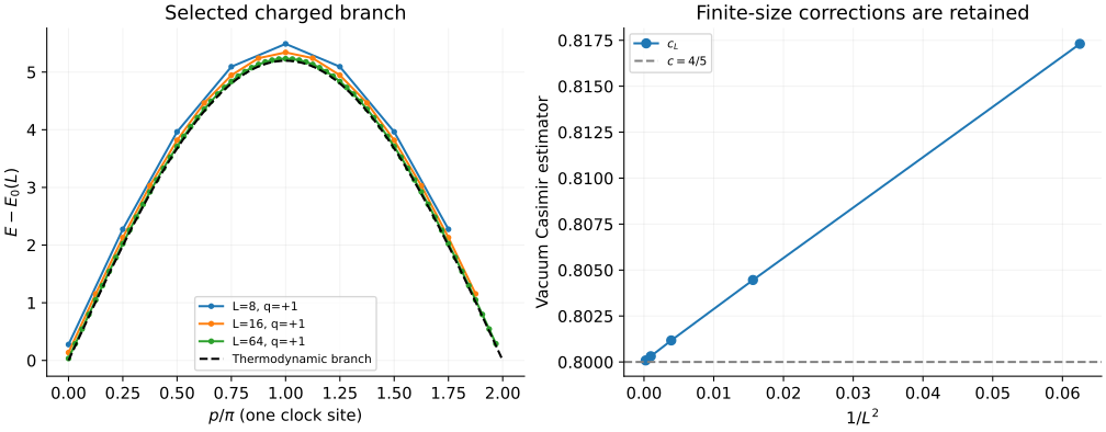
Potts charged gaps at three ring lengths approach a sinusoidal branch; the vacuum Casimir estimator approaches four fifths.

The left panel plots q=+1; q=-1 lies exactly on top of it. Every gap subtracts the same-length independently solved vacuum, not the extensive estimate \(Le_\infty\). The dashed curve is the thermodynamic limit

\[ \epsilon(p)=3\sqrt3\sin(p/2),\qquad 0\le p\le2\pi. \]

It is a reference curve, not a fit to the finite-size data. In particular, the finite ring has a positive charged gap at k=0, whereas the limiting branch is gapless. The sampled momenta stop at k=L-1: k=L would duplicate k=0.

Two different symmetries are visible:

Charge conjugation pairs q=+1 with q=-1 at the same k.
Reflection pairs k with L-k within a given charge.

At even L, k=L/2 is its own reflection partner. There are still two charge rows there, not four. The export has 2L+1 rows, including the vacuum, not the full \(3^L\)-dimensional spectrum.

To calculate only the first charged momentum of one charge:

bethe-potts-pbc 64 --branch charged --charge 1 --momentum-index 1 \
  --csv-table levels=potts-first-descendant.csv

The vacuum is still solved for subtraction even though its row is not shown. No spectral weights are supplied: an energy line alone does not tell us how strongly a local clock operator couples to it.

3. Extract finite-size estimators, not exact finite-size dimensions¶

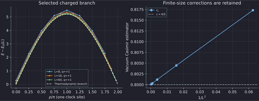
The right panel uses the vacuum energy:

\[ c_L=-\frac{6L(E_0-Le_\infty)}{\pi v},\qquad x_L=\frac{L(E-E_0)}{2\pi v}. \]

The first estimator approaches c=4/5. The charged k=0 level approaches x=2/15; k=1 and L-1 approach the first descendants, x=17/15.

L	Vacuum \(c_L\)	Charged k=0 \(x_L\)	Charged k=1 \(x_L\)
8	0.80445927	0.13508379	1.11427066
16	0.80117268	0.13417582	1.13057791
32	0.80031294	0.13377638	1.13382789
64	0.80008476	0.13357746	1.13414224
Limit	0.8	0.13333333	1.13333333

Finite-size corrections need not approach their limit monotonically: the k=1 values already illustrate that. Plotting against \(1/L^2\) is a useful display, not a claim that a single quadratic correction fits every level. The Bethe residual measures equation convergence, not the difference from CFT.

For an MPS comparison, first reproduce the finite-L energy in the matching charge/momentum sector. Only then study scaling with L or bond dimension. An enlarged MPS unit cell folds physical momenta; the exported k still refers to the original one-clock-site translation.

4. Why this is not an arbitrary XXZ spectrum¶

Internally, the solver uses L real roots of a twisted auxiliary XXZ chain with 2L spin-half sites and \(\Delta=\sqrt3/2\). The energy map is

\[ E_{\mathrm{Potts}}=2\sqrt3\,E_{\mathrm{XXZ}}+\frac L2. \]

The vacuum and charged family have different auxiliary twists and selected labels. Their physical identification is essential: a converged arbitrary twisted-XXZ solution need not occur in the Potts spectrum. The representations of the shared Temperley–Lieb algebra are different; see Fukai et al. and the selection audit.

--branch all means all supported families, not all excitations. Neutral excited states, other charged families and generic complex-root enumeration are not implemented. These roots are also not the direct Potts paper's complex-root and ghost-species bookkeeping.

5. Reproduce and validate¶

Download the native levels exports: L=2, L=4, L=8, L=16, L=32, L=64.

With the plotting dependencies, from the source checkout:

python3 scripts/plot_potts_qg_tutorial.py --check
python3 scripts/plot_potts_qg_tutorial.py
# Optional: regenerate this and the non-Hermitian XXZ tutorial.
python3 scripts/plot_potts_qg_tutorial.py --solver-dir /path/to/bethe/bin
# Optional independent clock/spin matrices; requires NumPy.
python3 scripts/plot_potts_qg_tutorial.py --check --oracle
python3 -m unittest discover -s scripts -p 'test_tutorial_potts_qg.py'

The script checks provenance, convergence, both symmetries, row counts, momentum and gap normalization. The tests add exact L=2 energies, scaling limits and deliberately corrupted/missing data. The optional oracle builds independent L=2,4 clock Hamiltonians and resolves charge and momentum; it does not use the Bethe equations or the CFT predictions.

Exports with failed levels or failed vacuum subtraction must not enter the plot. Native long-double and optional MPLAPACK fp128 are available when precision matters, but higher precision does not remove finite-size corrections or extend the selected physical family.