TASEP: relaxation, oscillation and finite-size scaling¶

All tutorials · Model guide · ASEP tutorial

Bethe ansatz also solves stochastic generators. In the totally asymmetric simple exclusion process, particles hop clockwise around a ring, but cannot land on occupied sites. The interesting spectrum describes how a probability distribution relaxes, rather than the energies of a quantum Hamiltonian.

This tutorial extracts a relaxation time, distinguishes it from an oscillation frequency, and compares fixed-density rings with a single-particle limit. All plotted points come from bethe-tasep-pbc exports.

1. Read the eigenvalue with the right sign¶

There are L sites, N particles and right-hop rate r. The convention is

\[ \frac{dP}{dt}=MP,\qquad \lambda=-g+i\omega,\qquad g\gt0,\quad\omega\ge0. \]

Columns of M sum to zero; off-diagonal entries are allowed transition rates. The stationary eigenvalue is zero. A nonstationary eigenmode evolves as \(e^{-gt}e^{i\omega t}\). The conjugate partner makes a real oscillatory contribution to P. Its decay time is \(\tau=1/g\), not \(1/|\lambda|\). The frequency is angular frequency, in radians per unit time; divide by \(2\pi\) for cycles per unit time.

bethe-tasep-pbc 16 --particles 4 --rate 1 \
  --csv-table relaxation=tasep-mode.csv --csv-table roots=tasep-roots.csv

The result has approximately

\[ \lambda=-0.10133095+0.22216778i,\qquad \tau\simeq9.87. \]

Do not add the imaginary part to the positive gap. Nor is frequency a momentum column: the tool selects the nonnegative-frequency representative without assigning a directed momentum in the user's original particle sector. Both real and imaginary parts have inverse-time units, not quantum-energy units.

2. Grow the ring at fixed density¶

Run half-filled and quarter-filled rings of sizes 8, 16, 32, 64 and 128:

for L in 8 16 32 64 128; do
  bethe-tasep-pbc "$L" --particles "$((L/2))" --rate 1 \
    --csv-table relaxation="half-${L}.csv"
done

The reproduction script also runs quarter filling and N=1, exporting roots alongside the mode. It validates those roots before saving any regenerated data.

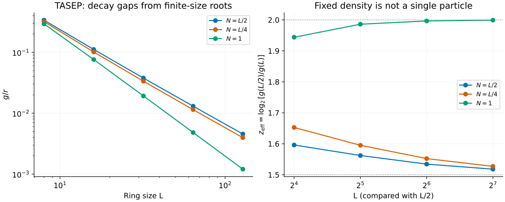
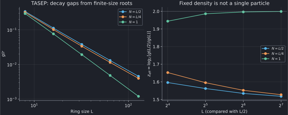
TASEP gaps for half filling, quarter filling and one particle, with local finite-size exponents.

For fixed density \(0\lt\rho=N/L\lt1\), the large-L relaxation gap scales as \(g\propto L^{-3/2}\), the one-dimensional Kardar–Parisi–Zhang dynamical exponent. The right panel uses successive calculated sizes,

\[ z_{\mathrm{eff}}(L)=\frac{\log[g(L/2)/g(L)]}{\log2}, \]

not a multi-parameter fit. At L=128 it gives about 1.518 for half filling and 1.527 for quarter filling. These are finite-size estimates approaching 3/2, not claims that the exponent has already reached its limit. The periodic gap analysis is due to Gwa–Spohn; the arbitrary-density result is derived by Golinelli–Mallick. The frontend solves their finite-size relaxation branch rather than inserting an asymptotic power law into the plotted points.

Holding N=1 fixed is a different limit: the density tends to zero. The single particle makes a directed random walk, with exact leading eigenvalue

\[ \lambda=r\left(e^{2\pi i/L}-1\right),\qquad g=2r\sin^2\frac\pi L\sim\frac{2\pi^2r}{L^2}. \]

That is why the green curve approaches exponent 2, about 1.99913 in the last size ratio. Exclusion-driven collective relaxation and dilute one-particle diffusive decay should not be compared as if they had the same size scaling.

3. Separate decay from drift¶

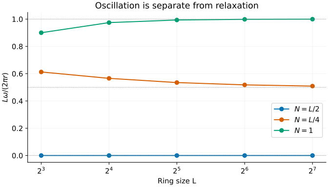
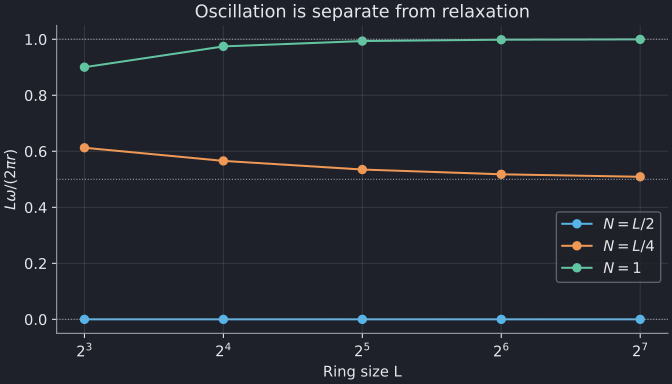
Rescaled angular frequency tends to one half at quarter filling, is zero at half filling, and tends to one for a single particle.

The large-ring fixed-density prediction is

\[ \omega\sim\frac{2\pi r}{L}|1-2\rho|. \]

At quarter filling the displayed rescaled frequency approaches 1/2; at half filling the selected leading eigenvalue is real. The single-particle curve instead follows the exact sine in the preceding formula and tends to 1. The horizontal guides label limits, not fitted curves.

A nonzero frequency means the mode oscillates while decaying. It does not mean the stationary state oscillates, and its absence does not mean the relaxation gap vanishes. The half-filled gap in the first figure is positive at every displayed finite size.

4. Symmetries, roots and tensor-network comparisons¶

Doubling r doubles g and the frequency and halves the relaxation time. The saved r=2 example checks this directly. Particle–hole symmetry also makes the reported mode at N=12 agree with N=4 on a 16-site ring. This statement uses the nonnegative-frequency convention; it is not a statement about the sign of a directed travelling mode.

The optional roots are fugacities, not physical momenta:

\[ Z_j=2/z_j-1,\qquad n=\min(N,L-N),\qquad \lambda=\frac r2\sum_{j=1}^{n}(Z_j-1). \]

Thus the N=12 export has four roots. The plotting script reconstructs the eigenvalue, checks the original fugacity equations and the first-harmonic translation factor. A small residual supports the selected solution; it does not prove completeness of a non-Hermitian spectrum.

For a tensor-network calculation of this generator, match periodic boundaries, particle number, hopping rate and the dP/dt=M P sign convention. If the code instead diagonalizes H=-M, negate the complex eigenvalue before comparing. An ordinary Hermitian variational energy minimization is not automatically a solver for this nonsymmetric generator. These tools supply neither left/right eigenvectors nor mode amplitudes in a chosen observable.

Finally, N=0 and N=L each have just one configuration. The calculation succeeds with has_mode=false and missing gap/frequency cells. That is absence of a nonstationary mode, not a zero relaxation gap or a failed solve. Conversely, an exhausted iteration budget exits with failure and must not be plotted.

5. Reproduce and check¶

Each link below is an original export with provenance and numerical status:

L	Half filling: mode / roots	Quarter filling: mode / roots	One particle: mode / roots
8	mode / roots	mode / roots	mode / roots
16	mode / roots	mode / roots	mode / roots
32	mode / roots	mode / roots	mode / roots
64	mode / roots	mode / roots	mode / roots
128	mode / roots	mode / roots	mode / roots

Additional checks: r=2 mode / roots; N=12 mode / roots; N=0 mode / empty roots; N=L mode / empty roots; L=5, N=2 mode / roots.

From the source checkout, with the plotting dependencies:

python3 scripts/plot_exclusion_tutorial.py --check
python3 scripts/plot_exclusion_tutorial.py
# Optional: regenerate both TASEP and ASEP examples with native executables.
python3 scripts/plot_exclusion_tutorial.py --solver-dir /path/to/bethe/bin
python3 -m unittest discover -s scripts -p 'test_tutorial_exclusion.py'

The shared script rejects incomplete rows, wrong signs, inconsistent roots and mismatched provenance. The tests check analytic limits, rate and particle–hole symmetry, and a separate ten-configuration Markov matrix for L=5, N=2. They also ensure that empty sectors cannot silently become zero-gap points. Plots use native fp64 results; long-double and optional MPLAPACK fp128 are available through the frontends when more precision is needed.