q-bosons: deforming the hopping, not adding a Hubbard U¶

View this page on GitHub

The q-boson chain offers a small, controlled benchmark for a bosonic MPS: keep particle number fixed, change the hopping matrix elements, and follow the spectrum from free bosons to the phase model. It is not the ordinary Bose–Hubbard chain, and its strong-deformation limit does not forbid double occupancy.

We will use three particles on five periodic sites, small enough to enumerate every canonical mode pattern and inspect the Bethe roots too.

1. Build the right local operator¶

The Hamiltonian and lowering matrix elements are

\[ H=-\sum_j\left(B_j^\dagger B_{j+1}+B_{j+1}^\dagger B_j-2N_j\right), \qquad B|n\rangle=\sqrt{[n]_q}\,|n-1\rangle, \]

\[ [n]_q=\frac{1-e^{-2\eta n}}{1-e^{-2\eta}},\qquad q=e^\eta,\qquad\eta\geq0. \]

Hopping and lattice spacing are one. \(N_j\) is the ordinary occupation operator, not \(B_j^\dagger B_j\). The deformation changes hopping amplitudes according to the local occupations; it does not introduce an on-site \(U n_j(n_j-1)/2\) term.

At eta=0, take the continuous limit \([n]_q=n\): ordinary free bosons.
At finite eta, occupation-dependent hopping gives an interacting integrable model.
--phase selects the exact infinite-eta limit, with \([n]_q=1\) for \(n\gt0\). Occupations 2, 3 and higher are still allowed.

For a fixed total of three particles, an MPS local basis 0,1,2,3 is enough to represent the whole sector. Truncating it to 0,1 would solve a different, hard-core model. For larger particle numbers, revisit that local cutoff.

2. Scan a small sector at three deformations¶

bethe-q-boson-pbc 5 --particles 3 --eta 0 --excitations all
bethe-q-boson-pbc 5 --particles 3 --eta 0.5 --excitations all
bethe-q-boson-pbc 5 --particles 3 --phase --excitations all

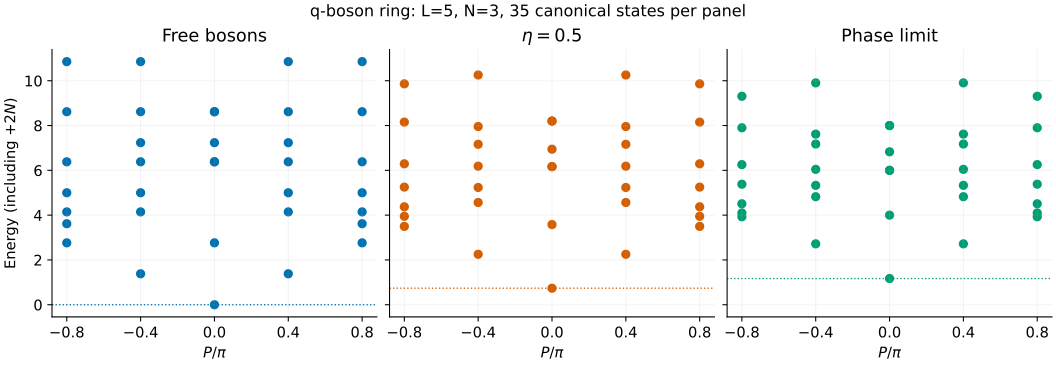
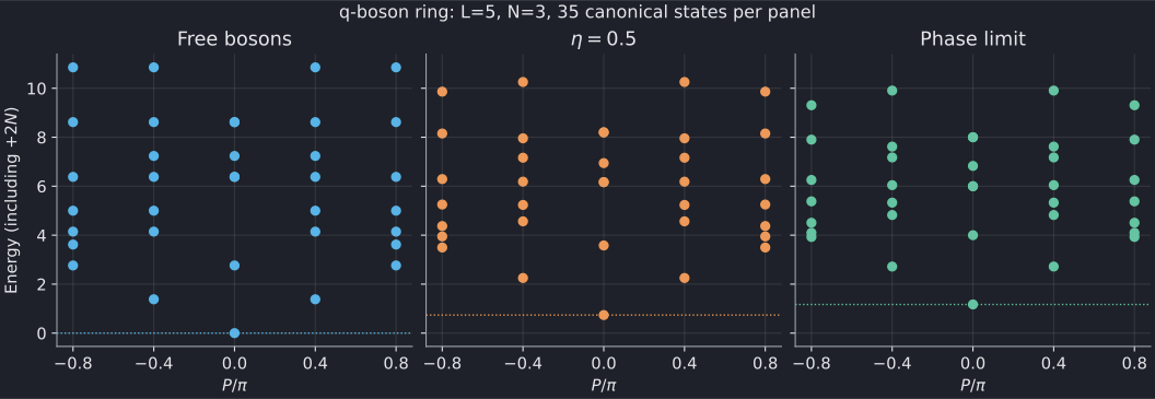
Five-site, three-particle spectra from free bosons to the phase limit

Each panel contains 35 canonical states; degenerate dots can overlap. The dotted horizontal line is the ground energy. The vertical axis shows absolute energy including the frontend's +2N shift, not the gap. At fixed particle number, subtracting \(2N=6\) converts these energies to a Hamiltonian with only the hopping terms. Excitation gaps within this sector are unchanged by that subtraction.

Download the three tables for each calculation:

Deformation	States	Ground reference	Roots
Free	CSV	CSV	CSV
eta=0.5	CSV	CSV	CSV
Phase	CSV	CSV	CSV

The physical momentum is reported in \((-\pi,\pi]\). On five sites its allowed values give the five vertical columns in each plot. Root momenta use a different, lifted convention; do not confuse them with the total momentum.

3. See the ground roots spread¶

Export auxiliary tables without requiring a root table on screen:

bethe-q-boson-pbc 5 --particles 3 --eta 0.5 --excitations all \
  --csv-table states=states.csv --csv-table reference=reference.csv \
  --csv-table roots=roots.csv

Join tables through state_id. The ground reference has its own ID, distinct from the ranked copy of the ground state in states; its root rows occur in the same roots export. root_index orders roots within each state.

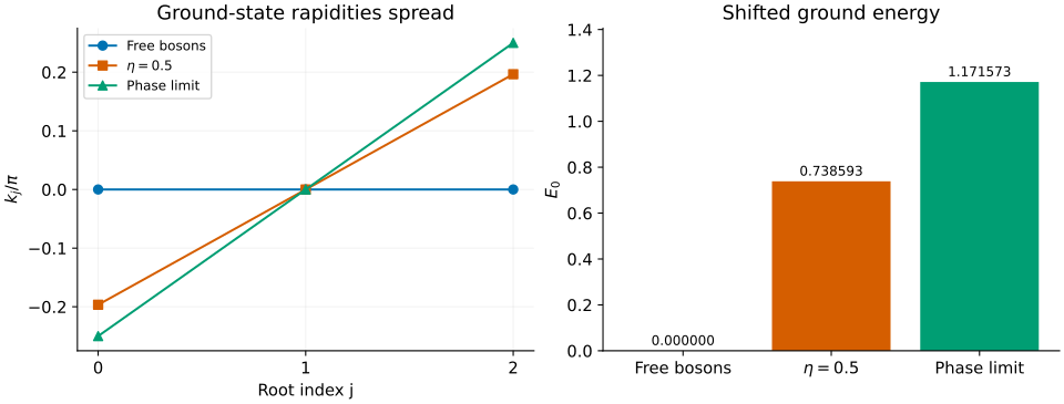
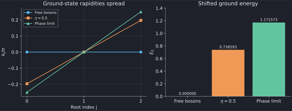
Ground rapidities and ground energy in the three deformation regimes

All ground roots coincide at zero in the free limit. At finite deformation they spread symmetrically, even though the total momentum remains zero. The interacting roots are spectral coordinates, not the occupation numbers of bare momentum orbitals.

In the phase limit the ground roots have a particularly simple form:

\[ k_j=\frac{2\pi I_j}{L+N},\qquad I_j=j-\frac{N-1}{2}. \]

For \(L=5,N=3\), they are \(-\pi/4,0,\pi/4\). Using the spectral energy rule \(E=\sum_j4\sin^2(k_j/2)\) gives \(E_0=4-2\sqrt2\simeq1.171573\). The finite eta=0.5 export lies between the free and phase ground energies, at approximately 0.738593. These values are useful normalization checks for an independently constructed MPO.

4. What has been enumerated?¶

Canonical states are labelled by sorted integer modes \(0\le m_0\le\cdots\le m_{N-1}\lt L\). Repeated modes are allowed. Their number is

\[ \binom{L+N-1}{N}=\binom{7}{3}=35 \]

for this example—the same as the fixed-N bosonic occupation-space dimension. Hard-core bosons would have only \(\binom{5}{3}=10\) states, underscoring why the phase limit must not be interpreted as a hard-core constraint.

The Bethe labels are \(I_j=m_j+j-(N-1)/2\). At eta=0 the roots are simply \(2\pi m_j/L\); at nonzero eta they deform continuously. The m and deviation columns preserve that representation even when very weakly split roots would round to the same printed k.

--excitations all visits every canonical pattern, but a matching candidate count alone is not proof that a numerical calculation succeeded. Check the converged count, aggregate outcome, row statuses and ground reference. A failed candidate is excluded from the ranked table and makes the scan incomplete. A missing gap is not zero.

Our small-sector implementation is checked against independent occupation- basis diagonalization in the model tests. The tutorial adds checks of canonical labels, the free and phase formulas, and the first two spectral moments computed directly from the occupation-basis hopping. Those moments provide a separate test of the Hamiltonian normalization.

The enumeration grows rapidly. --excitations 5 retains five levels but still solves the whole family; --max-candidates limits that work. This tool does not calculate form factors, spectral weights, quenches or open boundaries.

5. Reproduce the figures¶

With the optional plotting environment:

python3 scripts/plot_q_boson_tutorial.py
# Regenerate all nine named-table exports:
python3 scripts/plot_q_boson_tutorial.py \
  --solver bethe-q-boson-pbc
python3 scripts/plot_q_boson_tutorial.py --check
python3 -m unittest discover -s scripts -p 'test_tutorial_q_boson.py'

These examples use fp64. Long-double and fp128 can help resolve weak deformations, but neither higher precision nor a small residual repairs an incorrect local operator or Hilbert-space truncation.