XXX: from excitation energies to spectral weight
An energy level tells us where a response could appear. Its form factor tells us how strongly the chosen operator excites it. This tutorial adds that missing information to the finite-ring XXX scans, using the zero-field two-spinon triplet family.
1. Export a finite-ring spectrum
bethe-xxx-structure-factor 64 --csv xxx-spectrum.csv \
  --csv-table moments=xxx-moments.csv
The default channel is \(S^{zz}\), with spin-1/2 operators, \(H=\sum_j\mathbf S_j\cdot\mathbf S_{j+1}\), periodic boundaries, and J=1. All 528 states in the supported family are included. Each exported row is a delta-function line:
q is the momentum transferred by the operator, not an absolute excited
state momentum. weight is w, without the factor \(2\pi\). A line has no
height until we choose a broadening kernel or bin width.
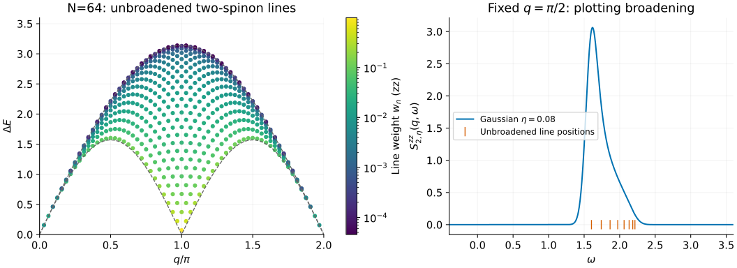
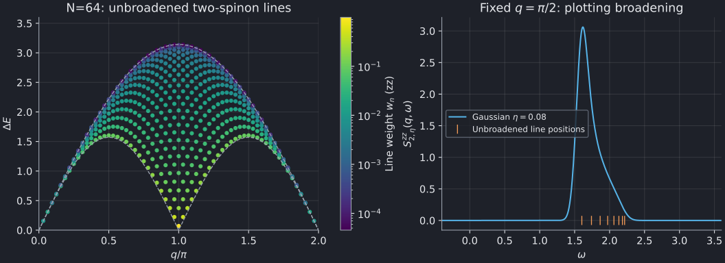
The left panel shows the unbroadened lines with color encoding their weights. The dashed curves are infinite-chain two-spinon boundaries, \(\omega_L=(\pi/2)|\sin q|\) and \(\omega_U=\pi|\sin(q/2)|\), provided as kinematic guides, not finite-N bounds. The right panel uses the exact finite momentum q=π/2, so it does not mix neighboring momentum bins.
Downloads: N=64 spectrum and moment sums.
2. Broaden only when plotting
For the right-hand plot we use a normalized Gaussian of width η=0.08:
Changing η changes the visual resolution, not the underlying line weights. The plotting script includes negative frequencies in the displayed Gaussian tails and enough range above the last line; broadening is not a physical negative-frequency response. There is no broadening option in the solver.
For an MPS dynamical spectrum, match the Fourier normalization, Hamiltonian, chain length and boundary condition before comparing areas or peak heights. For iMPS, these finite-ring data are useful checks, but increasing N is a separate convergence study. The continuum boundaries alone do not determine intensities, and multiparticle states outside this family are still absent. The separate thermodynamic tutorial now provides the exact infinite-chain two-spinon density without artificial broadening.
3. The whole momentum–frequency plane
For a more resolved demonstration, increase the ring to N=256 and include all 8,256 two-spinon states:
bethe-xxx-structure-factor 256 --csv xxx-n256-spectrum.csv \
  --csv-table moments=xxx-n256-moments.csv
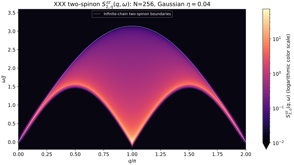
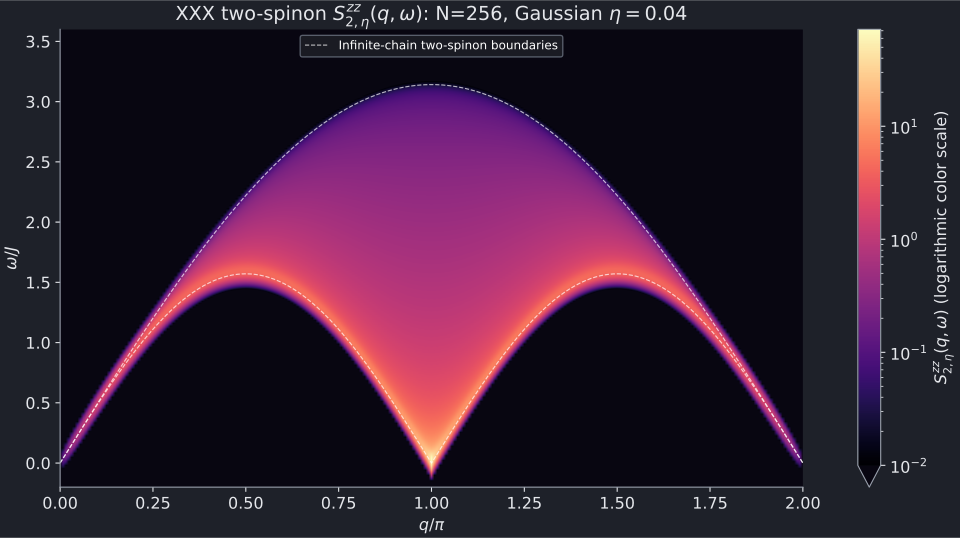
Full-resolution figure: light · dark · Download spectral lines · Download moment sums
This is the entire momentum range of the two-spinon contribution, not the complete many-spinon spectral function. It uses the same normalized Gaussian as above, now with \(\eta=0.04J\) (standard deviation; FWHM ≈0.094J). We sample frequency every 0.002J and keep all 256 exact momenta, spaced by \(\Delta q=2\pi/256\). There is no momentum broadening or interpolation: each narrow column shows one finite-ring momentum. The q=0 column is repeated at 2π only to close the periodic plotting edge, not counted twice in any sum.
The logarithmic color scale reveals weak spectral weight inside the continuum without losing the strong lower-edge response. Intensities below 0.01 use the dark background; this is only a display threshold, not a cut on exported weights. White dashed curves mark the infinite-chain two-spinon boundaries. The blurred intensity outside them, including negative frequencies near q=π, comes from Gaussian tails and finite-size effects—not additional states.
Compared with N=64, this gives four times the momentum resolution and halves
the broadening. Making η still smaller mainly exposes individual finite-ring
lines; a denser image grid alone cannot create better physical resolution.
For larger rings, --threads N parallelizes both root solving and form factors
using Uni20's scheduler. See parallel calculations
for an N=512 command and the library interface. The published N=256 image
does not depend on the worker count.
The N=256 family captures 94.89% of the integrated weight and 92.75% of
the first moment. These are the actual finite-ring fractions, without
renormalization; they need not match the N=64 percentages below.
4. Read coverage, not just convergence
The full zz integrated sum rule is
The N=64 export gives about 97.71% of this full weight, and 96.22% of the
full first-frequency moment. The moments table shows where that first-moment
coverage varies with momentum. Successful convergence means every state
in the requested family succeeded, not that the full DSF has been obtained.
Missing weight must not be hidden by rescaling the curves. Thermodynamic
two-spinon percentages are not finite-N normalization conditions either.
Try an independent small example:
bethe-xxx-structure-factor 4 --channel raising --diagnostics
In this channel the weights at q=π/2, π, 3π/2 are 1/3, 4/3, 1/3. Dividing by N gives 1/2, so this small ring exhausts the raising-channel sum rule. The zz weights are exactly half as large. That complete small example should not be generalized to arbitrary ring lengths.
5. Reproduce or inspect the calculation
From the source checkout with the plotting environment:
python3 scripts/plot_xxx_structure_factor_tutorial.py
python3 scripts/plot_xxx_structure_factor_tutorial.py --solver bethe-xxx-structure-factor
# Regenerate only the larger-ring heat map:
python3 scripts/plot_xxx_structure_factor_tutorial.py --heatmap-only --solver bethe-xxx-structure-factor
The first command reads the checked-in exports; the second replaces them with fresh N=64 and N=256 runs and reproduces both figures. The reference N=256 run took about three minutes on the development desktop; plotting saved data requires no Bethe solves. The parser checks channel, normalization, complete candidate counts, momentum selection, positive weights, sum-rule coverage and agreement between line sums and moment tables.
For selected-precision root/form-factor diagnostics and a derivation of the
normalization, see the structure-factor guide.
--references lists the determinant and sum-rule literature. The calculation
uses the normalized form factors of
Caux, Hagemans and Maillet;
it does not use continuum weights as substitutes for finite-state matrix elements.