Resolving six spinons with importance sampling
Two-spinon spectrum · Four-spinon quadrature · Selected-sector options
Six spinons contribute both inside and above the two-spinon band. Their large kinematic bandwidth does not mean that most of their intensity lies at high energy. To compare their response with an iMPS calculation, we need the spectral density, including contributions from configurations containing very soft spinons.
We use the infinite spin-\(1/2\) antiferromagnetic XXX chain at zero temperature and field, \(H=J\sum_j\mathbf S_j\cdot\mathbf S_{j+1}\), with \(J=1\). The output is the unbroadened longitudinal density \(S^{zz}_6(q,\omega)\). Frequency integrals use \(d\omega/(2\pi)\). The physical normalization is already included; no multiplier is fitted to a sum rule or another calculation.
Choose the scale of calculation
The hands-on tutorial uses two small calculations. Start with the native
long-double example to learn the command and output, then use the single-point
example with precision retries to examine soft spinons, sampling errors and
numerical controls.
| Calculation | Purpose | Measured cost |
|---|---|---|
| Three-frequency example, \(R=8\) | Learn the workflow | 0.38 CPU seconds with x86 extended80 long double |
| Single point, \(R=256\) | Inspect sampling and numerical diagnostics | About 20 seconds with four workers; 68 CPU seconds |
| Reference dataset, \(R=1040\) | Reproduce the recorded spectrum and plot compact data | See the dataset-specific compute budget |
The first two examples have substantial sampling and cutoff uncertainty; they teach the method without resolving the full physical response. Their measured costs and checks are described below. The reference campaign is a separate, production-scale calculation, not a step required to work through this tutorial. Its complete compact results can be plotted without rerunning the integrations. Timings refer to the linked validation records; measure a small query on your machine before budgeting a grid.
Why sampling needs a physical proposal
Momentum and energy conservation determine two momenta after four rapidities are chosen. The integrator includes every momentum branch and both labelled solutions. Its proposal mixes a background distribution with distributions that place one or two pairs near soft configurations. The full mixture probability enters each weight, including overlapping ways to generate it.
This is ordinary Monte Carlo integration with independent replicate streams. Changing the proposal changes the distribution of work and statistical error, while preserving the target integral. Concentrating draws in one region is useful only if all required regions retain support and the complete proposal probability is used. The geometry guide describes the measure and balancing between different choices of the solved pair.
Start with an inexpensive calculation
This small calculation checks the workflow before extending the rapidity domain or requesting a resolved spectrum:
bethe-xxx-structure-factor-thermo --sectors 6 \
  --momentum 1.57079632679489661923132169163975 \
  --omega-min 1.8 --omega-max 2.2 --points 3 \
  --precision long-double --six-cutoff 8 --replicates 4 --samples 32 \
  --seed 42 --threads 2 --density-relative-tolerance 1e-5 \
  --density-absolute-tolerance 0 --density-terms 64 --density-tail-order 16 \
  --diagnostics --replicate-output --json small-slice.json
Why evaluate the form factor at two precisions?
You select one format with --precision; the program automatically chooses
a lower precision for an internal accuracy check. It does not run two separate
Monte Carlo integrations or draw a second set of random configurations.
For each supported spinon configuration, the program evaluates the same
form-factor density twice: once at a lower precision and once at a higher
precision, called the guard precision. Both evaluations start from the
same geometry coordinates, converted separately into their respective formats,
and use the same contour controls. The lower result is a fresh calculation,
not a rounded copy of the higher result.
This tests sensitivity to roundoff. The formula contains special functions and sums whose terms can nearly cancel; choosing a floating-point format alone does not tell us how many useful digits survive. The difference between the two results contributes to the arithmetic diagnostic, together with the kernel's roundoff indicators and a check of its scalar prefactor. The program uses the higher-precision value, not an average of the two.
For example, long-double on the tested x86 system compares a 53-bit double
evaluation with a 64-bit long double evaluation. With MPFR, the higher density
precision normally follows --precision bits-N; --density-guard-bits can lower it
independently of geometry precision. The comparison uses 64 fewer bits, with
a minimum of 24, so a 192-bit density guard gives a 128/192-bit pair.
The arithmetic diagnostic plus the estimated contour remainder must fit within \(\mathrm{atol}+\mathrm{rtol}\,|W_{\mathrm{high}}|\). The program repeats both precision evaluations with a larger contour budget, so a successful check uses four density evaluations in total. Both budgets must pass, and their higher-precision results must agree; the result from the larger budget is retained. Agreement is a numerical stability check, not a rigorous error bound. Disagreement can originate in the lower precision even when the higher result is accurate: it means the requested check has not passed, not that the higher format is necessarily inadequate. Neither check measures Monte Carlo sampling error or the weight excluded by the rapidity cutoff.
Choose arithmetic for your calculation
On a machine with native extended80 long double, this example completes in
0.38 CPU seconds. Its three densities agree with a 384-bit MPFR check within
\(3\times10^{-16}\) relative. The observed sampling errors are still 66–76%,
and cutoff 8 omits substantial soft weight: arithmetic agreement does not make
this small run an accurate physical spectrum. The
validation record contains
the numerical controls, hardware and measured costs.
Check bethe-info for the actual native formats on your platform. If
long-double fails a check, try --precision fp128 with the same seed,
frequencies, domain and tolerance before using MPFR. Where extended80 is
available, binary128 compares a 64-bit-significand long double result against
its own 113-bit result. The precision guide
explains the comparison selected on other platforms. Binary128 support needs
an appropriate build.
Changing the seed can change the precision requirement
More samples, a new seed or a larger domain can encounter harder configurations.
For example, this query with --seed 2 fails its arithmetic check in extended80
but completes with binary128 at the same tolerance. Its densities agree with
MPFR192 within \(1.5\times10^{-30}\) relative; see the
native comparison record.
This is a useful same-input check to repeat before increasing the sample count.
Keep failed results and use distinct output filenames for each comparison. Do not search for a passing seed or average only successful replicates. Choose an inner tolerance for the accuracy you need, then check against a stricter calculation. The development study collects the wider precision and seed scans separately.
Retry difficult configurations at wider precision
A larger calculation can use --six-precision-stages fp80,fp128,reference.
On the x86 build used here, each draw first attempts extended80 geometry and
its 53/64-bit density check.
If the numerical checks fail for a recoverable reason, the same draw is retried
with binary128 geometry and a 64/113-bit density check. A final reference
retry uses MPFR with the precision and density guard you specify. The stage
list requires the corresponding native formats in your build; omit an
unavailable native stage and keep reference last.
These are whole-observation retries, including geometry and every contributing
root. They preserve the exact random draw and full importance weight. An
accepted result replaces the previous attempt; results from different
precisions are not averaged. A terminal failure prevents a spectrum estimate,
and failed draws are never discarded or replaced with new random numbers.
The recovery table retains each stage's attempts, accepts, retries and work.
The two-precision density check above still operates within each stage. The
stage list adds a way to recover the difficult observations without computing
every draw in MPFR. With a stage list, --precision sets the MPFR reference,
accumulation and output precision; it does not describe the arithmetic used
for every accepted observation. The export records all these precisions.
Omit --six-precision-stages to use a fixed-precision calculation. This also
provides a reference check: rerun the same inputs without the stage list to
compare against MPFR for every observation, rather than just the retries.
Extend the soft domain
Use a build or installation with extended80, binary128 and MPFR enabled for this stage list. This decimal input denotes a point extremely close to \(q=\pi/2\); its exact string is retained for comparing runs.
q=1.5707963267948966192313216916397514420985846996875529104874722961539082031431045
bethe-xxx-structure-factor-thermo --sectors 6 \
  --momentum "$q" --omega 2 --exchange 1 --channel zz \
  --precision bits-512 --density-guard-bits 256 --six-cutoff 256 \
  --six-precision-stages fp80,fp128,reference --samples-per-task 128 \
  --replicates 16 --samples 128 --seed 7304 --threads 4 \
  --density-terms 256 --density-tail-order 24 \
  --density-relative-tolerance 1e-6 --density-absolute-tolerance 0 \
  --diagnostics --replicate-output --json point.json
From a build directory, prefix the executable with ./. The sample count is
per replicate, so this requests 2,048 draws. These settings define a finite
integration domain and numerical checks; they do not promise a particular
relative sampling error. The point is a starting calculation to inspect before
running a frequency grid.
This query completed in 20.1 seconds with four workers on a Xeon Gold 6254, using 67.8 CPU seconds. Of its 2,048 draws, 2,026 passed in extended80; 22 retried in binary128, and 11 of those required MPFR. The final reference uses 512-bit geometry and a 192/256-bit density comparison. Accumulation and output retain 512 bits regardless of the successful stage.
The complete query preserves the original MPFR control's replicate identities, root counts and final density-work counts. Its mean differs by \(2.1\times10^{-16}\) relative, and every replicate mean and maximum by less than \(6\times10^{-16}\). The installed-program validation record retains the commands, precision stages, comparison and measured costs. The sampling error remains 15.4%; faster arithmetic neither reduces that scatter nor recovers the omitted rapidity tail.
The spectrum table contains the density. The diagnostics table separates
sampling error from contour and arithmetic diagnostics. The replicates table
retains each mean, sample count, supported-root count and largest observation.
The recovery table counts work from every attempted stage, including rejected
attempts; the diagnostics table reports the final observation work. An
unsuccessful replicate prevents an estimate over the remaining replicates.
The accompanying analysis script independently checks all replicate identities and recomputes the reported mean and sampling standard error:
python3 scripts/plot_xxx_six_spinon_tutorial.py \
  --raw point.json --momentum "$q" --output point-check.json
Run the script from the source directory. It needs only Python's standard library for this check and refuses to overwrite an existing analysis file. It also reports the fraction of the accumulated weight supplied by the largest observation and by the largest replicate.
Read the errors before increasing the grid
For \(B\) complete, equally sized replicate means \(\bar S_b\), the reported sampling error is
This estimate measures the scatter that the run observed. A few large weights can dominate a small run, and an unsampled rare region does not appear in its error bar. Examine replicate scatter and influential observations, increase independent work, and check a different seed. Calibrate proposal choices on separate streams before using them for a validation calculation.
These controls answer different questions:
| Change | What the comparison tests |
|---|---|
| More independent draws/replicates | Sampling scatter and sensitivity to rare large weights |
Larger --six-cutoff |
Weight outside the current rapidity domain |
| More residue terms and higher tail order | Evaluation of the auxiliary contour sums |
Higher --precision |
Fixed-mode energy-surface arithmetic, or the final MPFR stage when retries are enabled; also density if no guard override is set |
Higher --density-guard-bits at fixed geometry |
Density arithmetic alone, with MPFR |
The density check uses \(\mathrm{atol}+\mathrm{rtol}\,|W_6|\). The relative term sets the scale for nonzero matrix elements; the absolute term supplies a floor near zero. For example, an absolute tolerance of \(10^{-30}\) would not request thirty-digit accuracy everywhere. These examples use a zero absolute floor and explicit relative tolerances. Passing this inner check does not bound sampling, integration or omitted-domain error.
The rapidity cutoff \(R\) restricts all six rapidities to \(|\beta_j|\le R\), where \(p_j=2\arctan(e^{\beta_j})\). Large \(|\beta_j|\) means a spinon near momentum zero or \(\pi\), with very little energy. Increasing \(R\) can therefore add weight inside the bright continuum; it does not merely extend the high-frequency tail. A small sampling error does not bound this omitted weight.
Compare cutoffs with common precision and sufficiently strong contour controls. When sample streams are shared, use their paired replicate differences rather than assuming independent errors for the difference. Keep a failed calculation as a failed record. A numerical failure or missed sampled support is not a physical zero.
For two exports differing only in cutoff, the script checks their controls and computes the paired difference and its standard error:
python3 scripts/plot_xxx_six_spinon_tutorial.py \
  --raw lower-cutoff.json --compare-raw higher-cutoff.json \
  --momentum "$q" --output cutoff-check.json
A small difference does not bound the weight beyond the larger cutoff. Both estimates can omit the same soft region.
Distinguish contour failures from arithmetic failures
The diagnostics identify which part of a calculation needs improvement.
For a contour-tail failure, increase --density-terms and
--density-tail-order, holding precision and sample identities fixed.
For an arithmetic failure, increase precision while holding the contour
controls fixed. Raising precision alone does not shorten a truncated contour
tail, and adding samples does not repair either failure.
Compare two successful sets of stronger controls on the same inputs before expanding the sampling budget. A larger sample can expose configurations that a small calibration did not encounter; every observation still needs its checks. Preserve each failed export and its reason. Numerical agreement on a fixed sample is separate from sampling and cutoff convergence.
When the geometry needs higher precision
The energy surface retains distances from momentum zero or pi separately from integer multiples of pi. This avoids subtracting a very soft endpoint displacement from a number of order one. The rapidity cutoff alone therefore does not set a large significand-bit requirement.
Near a degenerate solved pair, the roots and coarea Jacobian can still be
ill-conditioned. If geometry fails, repeat the same inputs at higher
--precision; raising --density-guard-bits alone does not change geometry.
MPFR can also refine a difficult solve locally. The
sector guide describes these checks.
Successful geometry must still be followed by density, contour and weighting
checks. A wider significand does not necessarily provide a wider exponent
range, and refinement cannot recover input digits already rounded away.
For a new calculation, hold the domain, contour budgets and sample identities fixed while comparing precisions. Then vary the other controls separately. Use reference-data settings when reproducing that dataset; they are not a minimum-precision rule for new calculations.
Keep the plotted data independently checkable
The compact format retains the full requested frequency grid and stores
numerical metadata once per run, together with spectrum, diagnostic and
replicate rows. Fixed-precision results use bethe-six-spinon-slice-v1; staged
precision results use bethe-six-spinon-slice-v2 and also retain every recovery
row, including unused stages and failed attempts. Both include each raw export's SHA256,
source revisions, cutoff, proposal controls and timing summary. Local command
paths are omitted. Raw observations and archives are not needed to redraw a
figure, and are not included in the compact file.
For the single-point example above:
python3 scripts/xxx_six_spinon_tutorial_data.py \
  --raw point.json --momentum "$q" --cutoff 256 \
  --frequency 2 --output six-compact.json
Repeat --raw for separate runs and --frequency for every requested node,
in increasing order. Decimal input frequencies are matched uniquely within the
export's recorded arithmetic-roundoff allowance. The reader returns the input
as omega and retains the rounded export coordinate as computed_omega; the
stored source rows remain unchanged. There is no interpolation, and ambiguous
matches are errors. The packer rejects duplicate frequencies and missing
nodes. An unavailable node needs an explicit record with omega, a failed
or unavailable status, a reason, and raw_sha256 (or null if no export
exists); supply that list using --unavailable records.json.
Both tutorial plotters can use
read_compact_slice(document, momentum=q, exchange='1') from the same module.
It recomputes the estimates through the sampling validator and returns ordered
points with their original controls. Unavailable points have s6: null and
sampling_se: null; they must appear as gaps, not zeroes or connecting lines.
These checks preserve the evidence for an estimate; they do not certify its
sampling or cutoff convergence.
To plot a compact slice, install the optional plotting dependencies and run:
python3 -m pip install -r docs/tutorials/requirements.txt
python3 scripts/plot_xxx_six_spinon_tutorial.py \
  --compact six-compact.json --momentum "$q" --figure six-slice.svg
This writes six-slice.svg and six-slice-dark.svg, each with linear and
logarithmic density panels. The points are unbroadened; joining lines only
guide the eye. Error bars show the sampling SE, excluding cutoff uncertainty.
Unavailable frequencies interrupt the curve. The two-, four- and six-spinon
upper boundaries are marked when they fall within the requested frequency
range. A single-point file is useful for checking the renderer, but a physical
line shape requires a resolved frequency grid.
Read the reference spectrum
The reference calculation extends the rapidity domain to \(R=1040\) and uses 32 independent replicates at each of sixteen frequencies. The left panel shows the density on a linear scale; the logarithmic scale on the right makes the weaker high-frequency response visible.
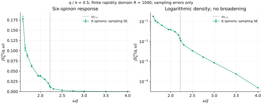
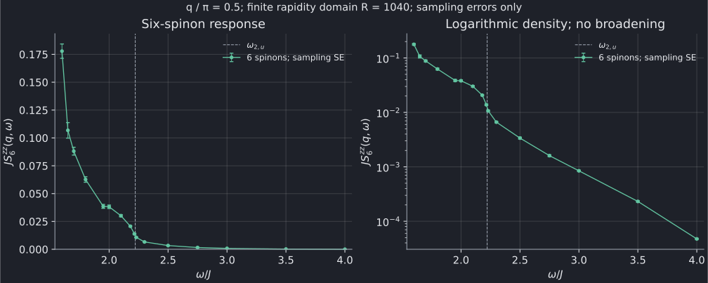
At this momentum the two-spinon band ends at \(\omega_{2,u}/J=\pi/\sqrt{2}\simeq2.2214\). Six spinons contribute on both sides of that boundary. The combined comparison puts this curve alongside the two- and four-spinon contributions and their partial sums. This frequency window ends at \(\omega/J=4\), well below the six-spinon upper edge; the final plotted point is not a band cutoff.
The symbols are the computed values, with no broadening or interpolation; joining lines guide the eye. Bars show the observed sampling standard error, which ranges from 2.49--6.52%. 15 of the sixteen points meet the initial 5% sampling target. The validation record retains the individual errors, influential-observation diagnostics and precision-retry counts. These are finite-domain estimates: the bars do not include the omitted rapidity tail or certify that rare configurations have been adequately sampled.
Redraw either theme directly from the compact data:
python3 scripts/plot_xxx_six_spinon_tutorial.py \
  --compact docs/tutorials/data/xxx-six-spinon-slice.json \
  --momentum 1.5707963267948966192313216916397514420985846996875529104874722961539082031431045 \
  --figure six-slice.svg
This command uses the saved estimates and runs no integrations. The optional production recipe gives the installed-program commands, predetermined sample streams and measured cost of recalculating the full dataset. The smaller examples above are sufficient to learn the workflow.
The six-spinon library interface provides independent geometry and recovery precision when needed. To obtain zeroth and first moments, use the direct moment calculation and its own domain checks; a sparse display grid is not a substitute for a frequency integral.