SU(n) fermions: components are not Bethe levels
All tutorials · Model guide · Gaudin–Yang tutorial
Adding internal components lets fermions share spatial orbitals without violating antisymmetry within any one component. Contact repulsion then couples the components. This tutorial follows a three-component gas and shows how physical populations become a hierarchy of auxiliary Bethe roots.
This is a continuum gas, not the SU(3)/ULS permutation spin chain. We use \(\kappa\) for the component count, N for particle number, and \(\ell\) for the physical circumference.
1. Start with nine particles, not nine lattice sites
All masses and all intercomponent repulsions are equal:
Same-component contact interactions vanish by antisymmetry. There are no component-dependent fields, traps or chemical potentials. Choose populations 3,3,3 and circumference 9, so the total density is one:
bethe-sun-fermions-pbc --populations 3,3,3 --length 9 --c 1 \
  --csv-table states=sun-state.csv --csv-table components=sun-components.csv \
  --csv-table roots=sun-roots.csv
The energy is approximately 7.77546038 and momentum is zero. The general solution is due to Sutherland; the finite nested equations used here are Eqs. (2)–(3) of Lee–Guan–Batchelor. Although that paper also develops thermodynamics, these examples solve finite-ring equations without a thermodynamic or string approximation.
2. Repulsion raises the charge energy
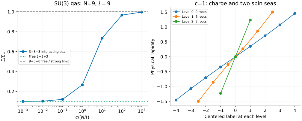
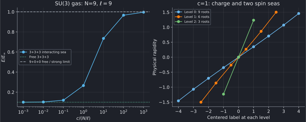
The left panel uses seven native calculations from c=0.001 to 1000, with dimensionless interaction \(\gamma=c/(N/\ell)\). Its reference energy is
At c=0 the three independent three-particle seas have energy \(8\pi^2/27\simeq2.92432723\). The weak-coupling slope counts pairs of different components:
At c=0.001 the shift is about 0.00599850. By c=1000 the energy is 29.14229213, close to the finite-ring strong-coupling limit. No power-law fit or extrapolation supplies these points.
The 9,0,0 sector is an exact free-fermion reference at every c. Since N=9 is odd, its periodic shell coincides with the charge shell of the displayed strong-coupling limit. This is deliberately different from the even-N shell subtlety in the Gaudin–Yang example.
3. Follow the nesting without losing physical component labels
For sorted occupied populations \(N_1\ge\cdots\ge N_\kappa\), the sea sizes are
Thus 3,3,3 produces 9 charge roots, 6 first-level spin roots and 3 second-level spin roots. Only level 0 contains the momenta whose squares enter E. Adding all levels' squared rapidities would overcount auxiliary degrees of freedom. The horizontal labels in the right panel belong to their respective seas; a label at one level is not the identity of a particle at another.
Try an imbalanced input with an empty component:
bethe-sun-fermions-pbc --populations 1,0,5,3 --length 9 --c 1 --roots
The physical component table remains in input order:
| Input component | Population | Nesting rank |
|---|---|---|
| 0 | 1 | 2 |
| 1 | 0 | absent |
| 2 | 5 | 0 |
| 3 | 3 | 1 |
Rank zero is the reference component. Empty components have no Bethe sea;
they are not assigned a spurious zero rank. The sorted occupied list is
5,3,1, giving sea sizes 9,4,1 and energy 10.10040293. The saved 5,3,1 run
has exactly the same roots and energy. Equal populations are sorted stably.
The additional 3,1,1,1 example exercises four occupied components, with
sea sizes 6,3,2,1.
4. Supported shells and cross-model checks
Every occupied component must have an odd population on the interacting
centered branch. Hence 3,3,3 is supported and 2,2,2 is not. This is a
restriction of the implemented periodic shell, not of the physical model's
integrability. Zero populations are allowed. Exact c=0, single-occupied-component
and vacuum paths allow arbitrary nonnegative counts.
Free components occupy integer momentum modes; even populations use a
positive-current representative when the shell is degenerate. For example,
2,0,2 at c=0 and circumference 1 has P=\(4\pi\). Continuum momentum is not
folded into a lattice Brillouin zone.
The saved data include several checks useful before an MPS comparison:
- Populations
3,3reproduce the separate Gaudin–Yang solver at the same circumference and coupling. - Populations
1,1,1form an antisymmetric internal singlet with a symmetric spatial ground state. Its charge roots and energy agree with three Lieb–Liniger bosons; the auxiliary roots still describe a different internal state, and generic observables need not agree. - Doubling circumference and halving c at fixed populations preserves \(\gamma\): all physical roots halve and E becomes one quarter.
Match the factor 2c, physical density and component populations when benchmarking a continuum discretization. The code does not supply arbitrary excited states, unequal masses, unequal pair couplings or attractive branches. If continuation stops early, an energy may belong to the last reached c: the requested coupling, reached coupling, both residuals and success status must agree before treating it as a target result.
5. Reproduce and validate
| c, populations 3,3,3 | State | Components | Roots |
|---|---|---|---|
| 0.001 | CSV | CSV | CSV |
| 0.01 | CSV | CSV | CSV |
| 0.1 | CSV | CSV | CSV |
| 1 | CSV | CSV | CSV |
| 10 | CSV | CSV | CSV |
| 100 | CSV | CSV | CSV |
| 1000 | CSV | CSV | CSV |
| Other calculation | State | Components | Roots or free modes |
|---|---|---|---|
| c=0, 3,3,3 | CSV | CSV | modes |
| 9,0,0 | CSV | CSV | modes |
| 5,3,1 | CSV | CSV | roots |
| 1,0,5,3 | CSV | CSV | roots |
| Rescaled 3,3,3 | CSV | CSV | roots |
| 3,3 | CSV | CSV | roots |
| 1,1,1 | CSV | CSV | roots |
| 3,1,1,1 | CSV | CSV | roots |
| Free even shell | CSV | CSV | modes |
| Vacuum | CSV | CSV | empty modes |
Reduction references: Gaudin–Yang state, charge roots, spin roots; Lieb–Liniger state and roots.
With the plotting dependencies, from the source checkout:
python3 scripts/plot_multicomponent_tutorial.py --check
python3 scripts/plot_multicomponent_tutorial.py
# Optional: regenerate both multicomponent tutorials and their reference runs.
python3 scripts/plot_multicomponent_tutorial.py --solver-dir /path/to/bethe/bin
python3 -m unittest discover -s scripts -p 'test_tutorial_multicomponent.py'
The script checks every nested equation, component mapping, sea size, energy reconstruction and continuation status. It retains the native export provenance. The tests add reductions, scaling, limiting slopes and corrupted-table checks. The default fp64 examples can be repeated manually with native long-double or optional MPLAPACK fp128; changing precision does not remove unsupported-shell restrictions.