Scaling Lee–Yang: a negative central charge and a positive particle gap
All tutorials · Model and numerical guide · Sine-Gordon comparison
The scaling Lee–Yang model is a particularly clean nonunitary example: it has one massive particle, yet its ultraviolet conformal theory has negative central charge. Here we calculate the periodic vacuum energy across scales, then follow a selected one-particle gap toward its infinite-volume mass.
These are continuum field-theory calculations. The tools do not construct a finite non-Hermitian spin chain, compute left/right eigenvectors, or measure matrix elements. Real energies in this example do not imply a unitary theory.
1. Which energy does the vacuum tool return?
Use particle mass m=1, circumference L and velocity=1:
bethe-lee-yang-vacuum --mass 1 --length 0.1 \
  --csv-table vacuum=ly-vacuum.csv
The useful dimensionless variable is \(r=mL\). The output separates the bulk-subtracted energy and its scaling function,
The tool does not supply an absolute bulk energy density. At r=0.1, it returns
\(Y\simeq-0.20835016\) and \(c_{\mathrm{eff}}\simeq0.39791949\).
Since L=0.1 here, the energy itself is approximately -2.08350158, not -0.20835.
The columns casimir_energy and scaling_function deliberately keep these
quantities separate.
2. Why does the plot approach +0.4 instead of -4.4?
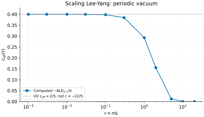
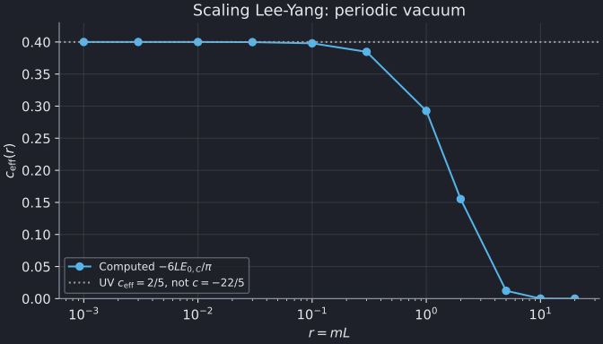
The ultraviolet CFT is \(M(2,5)\), with central charge \(c=-22/5\) and lowest left/right conformal weight \(h_{\min}=\bar h_{\min}=-1/5\). On a periodic circle, the lowest energy samples that negative-weight sector, not the identity sector:
Thus the positive coefficient extracted from the lowest energy is the effective central charge. To recover c, one also needs the conformal-sector information: \(c=2/5+24(-1/5)=-22/5\). Neither the sign of the vacuum energy nor a fit to its coefficient alone determines c. The finite-r curve is a computed scaling diagnostic, not a central charge at every circumference.
The model and finite-volume conventions are developed by Bajnok–el Deeb–Pearce, especially Eqs. (151)–(152), (212) and (218). In the small-r limit, \(Y\to-\pi/15\); at large r, the bulk-subtracted vacuum energy tends to zero. The markers are eleven separately converged TBA solves, not values from an interpolation formula. At r=0.001 the effective charge is within \(3\times10^{-7}\) of 0.4; that remaining finite-r difference is not solver noise.
3. Follow one massive excitation
The excited-state tool is a separate TBA calculation with quantized sources. For now it supports one zero-momentum regular branch at \(5\le mL\le30\):
bethe-lee-yang-excited --mass 1 --length 5 \
  --csv-table levels=ly-levels.csv --csv-table source=ly-source.csv \
  --csv-table gap=ly-gap.csv
The levels table contains the vacuum and one-particle Casimir energies. The
quantity to compare with an excitation calculation is instead
At m=1, L=5, the vacuum Casimir energy is about -0.0012816882 and the one-particle Casimir energy is 1.0293562331. Their difference is 1.0306379213. Replacing the gap by the excited row would lose a visible vacuum correction.
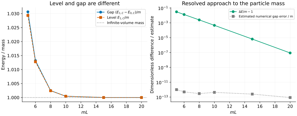
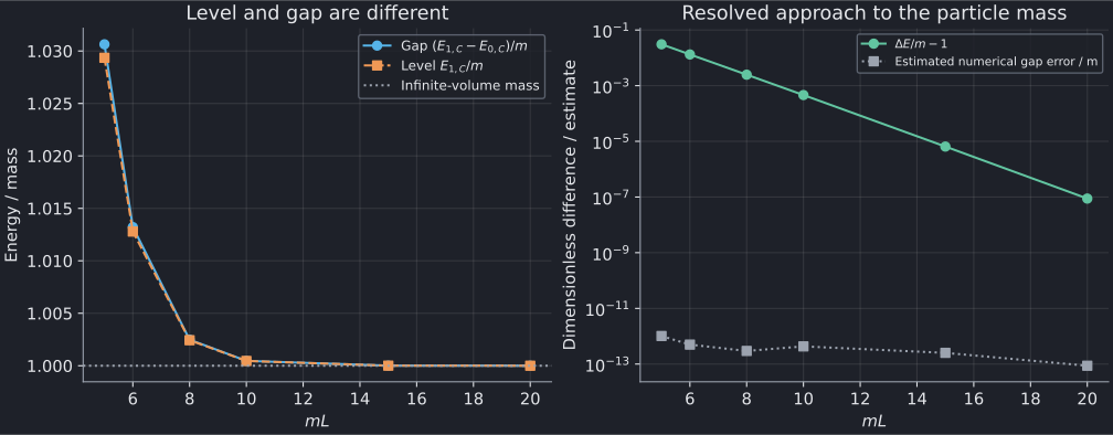
The right panel separates the physical finite-size correction from the estimated numerical error. At mL=20 the gap is still above m by roughly \(8.8\times10^{-8}m\), while the exported error estimate is about \(8.7\times10^{-14}m\). The estimate is not a rigorous interval bound, but these scales are well separated. Connecting lines merely guide the eye; no exponential fit or extrapolated mass is needed for this comparison.
Dorey–Tateo, Eqs. (2.3)–(2.7), derive the excited-state source construction by analytic continuation. Our implementation uses its regular infrared branch. The source table reports the imaginary source coordinate \(\beta\), its displacement from \(\pi/6\), and its quantization diagnostics. This beta is not sine-Gordon's coupling.
Do not continue the plotted curve toward the UV by ignoring the tool's domain check. The source configuration changes at smaller volume; the current solver does not implement that continuation. The vacuum UV calculation above is supported independently. Nor does changing a parameter in the source-free vacuum equation generate an excited level.
4. Match a non-Hermitian MPS calculation
The first figure is a finite-size energy benchmark, and the second a gap benchmark. For a lattice realization approaching this scaling theory:
- Identify the periodic sector and the lowest conformal weight before extracting c from finite-size energies. The coefficient alone gives an effective value.
- Match the physical mass, velocity and circumference. The exported theory uses velocity=1; a lattice energy scale and correlation length must be converted consistently before identifying r.
- Subtract the same ground-state energy when forming a gap. A fitted bulk energy density cancels between levels, but the finite-size vacuum term does not.
- Treat lattice corrections, finite-bond-dimension errors and TBA numerical estimates as separate sources of discrepancy. These energy tools supply no biorthogonal spectral weights or ordinary positive-norm interpretation.
A simple units test is m=2, L=1/2 versus m=1, L=1: r is unchanged, Y is unchanged, and the Casimir energy doubles. Likewise, the one-particle gap at m=2, L=2.5 is twice that at m=1, L=5. Saved exports check both transformations. The frontends support fp64, native long-double and optional MPLAPACK fp128; the tutorial uses fp64 throughout.
5. Reproduce and validate
Download the vacuum scans: 0.001, 0.003, 0.01, 0.03, 0.1, 0.3, 1, 2, 5, 10, 20, and the m=2, L=1/2 units check.
| mL (m=1) | Levels | Source | Gap |
|---|---|---|---|
| 5 | CSV | CSV | CSV |
| 6 | CSV | CSV | CSV |
| 8 | CSV | CSV | CSV |
| 10 | CSV | CSV | CSV |
| 15 | CSV | CSV | CSV |
| 20 | CSV | CSV | CSV |
The rescaled one-particle example also has separate levels, source and gap tables.
From the source checkout, with the plotting dependencies:
python3 scripts/plot_field_theory_tutorial.py --check
python3 scripts/plot_field_theory_tutorial.py
# Optional: regenerate both field-theory tutorials using native executables.
python3 scripts/plot_field_theory_tutorial.py --solver-dir /path/to/bethe/bin
python3 -m unittest discover -s scripts -p 'test_tutorial_field_theory.py'
The shared script preserves the individual runs' metadata, joins levels/source/gap from the same invocation, checks convergence and refinement diagnostics, and reconstructs the gap to catch energy-reference mistakes. Missing observables, non-finite values and failed statuses are rejected. The tests check UV/IR behaviour, mass scaling, a value from the independent vacuum oracle, and corrupted exports. The reference guide describes the independent quadrature and the meaning of each error estimate.