Doping the Hubbard chain¶

View this page on GitHub

At half filling we found gapless spinons but a charge gap. Now set \(n=N/L=0.75\), retaining \(U/t=4\), \(t=1\), zero field and zero temperature. This tutorial shows the doped elementary branches and how to choose the energy zero for an iMPS calculation of \(H-\mu N\).

Start with the half-filled tutorial for Hamiltonian normalization and the meaning of spinons and holons. This calculation uses the same executable; there is no finite chain length to choose.

1. Solve at a fixed density¶

bethe-hubbard-dispersion --u 4 --density 0.75 --points 129 \
  --convention symmetric --reference fermi --csv hubbard-doped-symmetric.csv

The solver determines the occupied charge sea and chemical potential from the requested density, then reuses that background for every point. It does not assume that the half-filled chemical potential still applies.

For this example the metadata gives

These differ by U/2 as expected. If your iMPS calculation uses a chemical potential to obtain this density, compare it with the value in the matching Hamiltonian convention.

2. Read the three branches¶

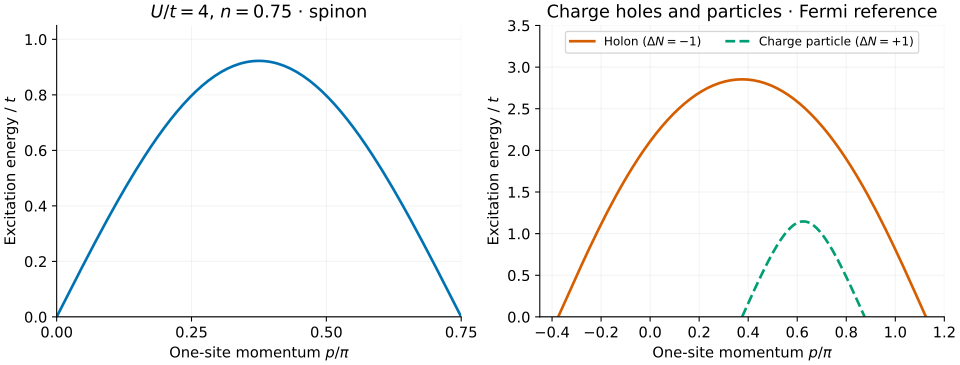
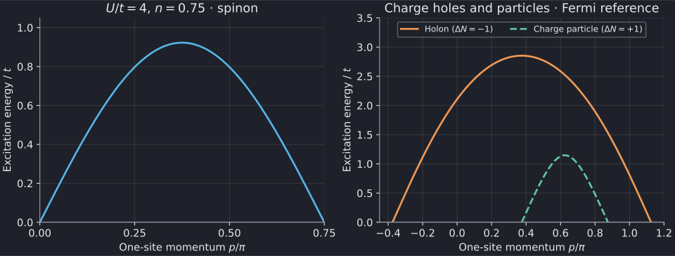
Full-size figure: light · dark.

All three branches have zero Fermi-referenced energy at their endpoints. The momenta are unwrapped one-site momenta, in this frontend's fixed convention:

The charge-particle adds a real charge root outside the occupied sea. It is not the half-filled antiholon: different branches are selected by --branch all at density one and below density one. The tool does not include the doped gapped string branches.

Use the p_over_pi column, not parameter, for these plots. In particular, the charge-particle's bare parameter jumps from π to −π in the middle of its grid, while its dressed physical momentum and energy remain continuous.

3. Separate the two energy choices¶

--convention chooses the interaction; --reference chooses whether to subtract the chemical-potential cost. They are independent options:

Unlike at half filling, the symmetric Hamiltonian difference alone is not Fermi-referenced. Its chemical potential is nonzero. The CSV includes both symmetric_energy and fermi_energy, so we can plot that difference directly:

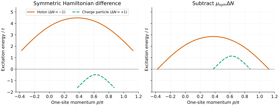
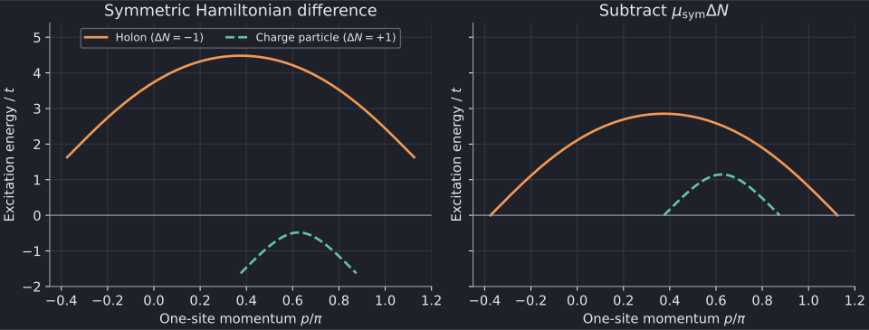
Full-size energy-reference comparison: light · dark.

At the charge-particle endpoints, the symmetric Hamiltonian cost is \(\mu_{\mathrm{sym}}\), approximately −1.62956 t. At the holon endpoints it is \(-\mu_{\mathrm{sym}}\), approximately +1.62956 t. Subtracting \(\mu_{\mathrm{sym}}\Delta N\) brings both to zero. Spinons have \(\Delta N=0\) and are unchanged.

As a consistency check, export with the other interaction convention:

bethe-hubbard-dispersion --u 4 --density 0.75 --points 129 \
  --convention unshifted --reference fermi --csv hubbard-doped-unshifted.csv

Its energy values agree with the first export: a consistently Fermi-referenced spectrum is convention-independent. The tutorial tests check this point by point, not just at the endpoints.

4. Avoid misleading momentum comparisons¶

The holon grid extends beyond π. That is intentional: the branch has a continuous unwrapped momentum coordinate. Keep it that way when first comparing with the exported plot.

If your MPS code reports the phase of translation by a cell of length \(\ell\), the conversion is

When plotting a folded curve, split it where the folded coordinate wraps; do not connect a jump across the zone or sort distinct folded branches into one line. Also check the domain-wall momentum gauge and choice of Fermi-point spectators. A universal momentum offset cannot be inferred from the cell length alone.

These lines supply elementary reference energies. They are not electron spectral functions or complete multiparticle thresholds; matching quantum numbers is essential before identifying an iMPS excitation with one of them.

5. Approach half filling with care¶

The limit from below is subtle. As \(n\to1^-\), the background chemical potential approaches the lower edge of the Mott plateau. At exactly \(n=1\), the half-filled tool chooses the plateau's middle instead. Comparing two Fermi-referenced plots without accounting for this different chemical potential can look like a discontinuity in the wrong quantity.

The real charge-particle interval also shrinks to a point:

It does not turn into the gapped antiholon band. Use the half-filled frontend mode for that branch, rather than extrapolating the doped particle curve.

Reproduce and extend¶

Download the symmetric and unshifted exports. Both use the Fermi reference. The shared Hubbard plotting script reproduces this tutorial and the half-filled one:

# From the source checkout, using the half-filled tutorial's Python environment:
python3 scripts/plot_hubbard_tutorial.py
python3 scripts/plot_hubbard_tutorial.py --check
python3 -m unittest discover -s scripts -p 'test_tutorial_hubbard.py'

The checks need no C++ build or Matplotlib. They verify branch labels, momentum ranges, convergence, chemical-potential shifts and gapless endpoints. The numerical exports retain their precision; conversion to Python float is only for plotting and these fp64 example checks.

For your own U or density, inspect Background status and every row's status. Do not plot empty failed-energy cells as zero. Weak coupling or extreme densities can require larger mesh budgets or higher precision; see the doped solver guide.

The background and dressed-energy equations follow Essler; particle/hole branch conventions are discussed by Luo–Pu–Guan. The reference guide fixes the precise momentum definitions.