Kondo response: subtract the host and calibrate the scale¶

All tutorials · Model guide · Central-spin tutorial

A lattice impurity calculation and a continuum Bethe-ansatz energy cannot always be compared directly. This tutorial chooses a well-defined universal quantity: the change in impurity-induced energy under a uniform field, together with its conjugate magnetization.

1. Specify what is being subtracted¶

The frontend describes the isotropic, antiferromagnetic, single-channel, spin-1/2 Kondo model at zero temperature in its scaling limit. The field acts on the impurity and host, with equal g factors:

\[ H_{\mathrm{field}}=-b(S_{\mathrm{imp}}^z+S_{\mathrm{host}}^z). \]

b is the full Zeeman splitting in energy units. Define

\[ \begin{aligned} E_{\mathrm{imp}}(b)&=E_{\mathrm{with\ impurity}}(b)-E_{\mathrm{clean\ host}}(b),\\{} \Delta E_{\mathrm{imp}}(b)&=E_{\mathrm{imp}}(b)-E_{\mathrm{imp}}(0),\\{} M_{\mathrm{imp}}&=-\frac{d\Delta E_{\mathrm{imp}}}{db}. \end{aligned} \]

The two host calculations must use the same field and host convention. The response includes the host magnetization change induced by the impurity; it is not simply the local expectation \(\langle S_{\mathrm{imp}}^z\rangle\). The distinction and the limits of absolute-energy comparisons are discussed by Barcza et al., Sec. VII.

bethe-kondo-response --field 2 --scale 1 --csv-table response=kondo.csv

This gives approximately \(\Delta E_{\mathrm{imp}}=-0.34629170\) and \(M_{\mathrm{imp}}=0.27516364\). The command does not take a bare exchange, bandwidth, chain length or boundary condition; it is not a finite-band solver.

2. Calibrate T_B before overlaying data¶

The positive --scale parameter is the energy \(T_B\), not an unspecified “Kondo temperature”. Its zero-field susceptibility fixes the convention:

\[ a_0=\frac1{\sqrt{2\pi e}},\qquad \chi_0=\left.\frac{dM_{\mathrm{imp}}}{db}\right|_0=\frac{a_0}{T_B}, \qquad T_\chi=\frac1{4\chi_0},\qquad T_B=4a_0T_\chi. \]

Thus a susceptibility measured with the same field/host subtraction gives \(T_B=a_0/\chi_0\). For T_B=1 the native output is χ₀≈0.2419707245. In the source paper's Eqs. (124)–(126), b=2B and T_B=2T₁. Missing either factor of two changes the susceptibility or energy derivative.

For an MPS benchmark:

Compute the impurity-induced total response using a uniform field and a matching clean host, not just the impurity site's polarization.
Check finite-size/bond-dimension convergence and determine χ₀ in the same units. It calibrates T_B without an assumed bare-exchange conversion.
Plot against \(x=|b|/T_B\) and compare the subtracted energy and response.

The scaling comparison requires both b and T_B to remain small relative to the host bandwidth. The very large x values below illustrate the continuum curve; they are not a promise that a chosen lattice bandwidth supports them.

3. Follow the crossover and slow saturation¶

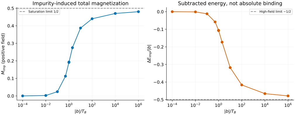
The impurity-induced magnetization approaches one half slowly; the energy change divided by field approaches minus one half.

All markers are native fp64 evaluations, including both sides of x=1. The line segments connect them; no interpolation supplies additional solver values. At small field,

\[ M_{\mathrm{imp}}=a_0\frac b{T_B}+O((b/T_B)^3),\qquad \Delta E_{\mathrm{imp}}=-\frac{a_0b^2}{2T_B}+O(b^4/T_B^3). \]

At b=0 both observables are exactly zero, while χ₀ remains finite; that point is included in the downloads but omitted from the logarithmic axes. Magnetization is odd in b, whereas energy change is even.

The high-field approach is slow: even at x=10⁶ the magnetization is only 0.48054872, not 1/2. The energy ratio is about -0.47880412, approaching -1/2. There is no finite-x saturation threshold in this universal curve.

The crossover x=1 is not a phase boundary. The implementation switches between accelerated series and Fourier-integral representations; the latter has a conditionally convergent tail at x=1. The numerical guide explains why a naive finite-cutoff integral can be misleading there.

4. Check signs, units and numerical errors¶

The downloads include b=-2 and the scale-transformed point b=6, T_B=3: the latter has the same x=2 and magnetization, three times the energy change, and one third the zero-field susceptibility.

Centered finite differences around b=1 and 2 verify the minus sign in \(M_{\mathrm{imp}}=-d\Delta E_{\mathrm{imp}}/db\). This differs from the central-spin tutorial's positive field term and derivative convention.

The exported magnetization_error is absolute in M; scaled_energy_error is absolute in \(\Delta E_{\mathrm{imp}}/|b|\), not in the physical energy or in \(\Delta E_{\mathrm{imp}}/T_B\). Away from zero field, multiply the latter estimate by |b| to express it in energy units. These estimates are convergence diagnostics, not rigorous interval enclosures.

Incomplete runs omit all physical observables and exit 2. Reject them rather than plotting missing responses as zero. Native long-double and optional MPLAPACK fp128 are available; neither changes the field convention or makes this a finite-temperature, multichannel, anisotropic or finite-band calculation.

5. Reproduce and validate¶

The response exports use T_B=1 unless stated otherwise:

Region	Native CSV files
Zero/low field	0, 0.0001, 0.01, 0.1, 0.5
Crossover	0.99, 1, 1.01, 2
High field	10, 100, 10000, 1000000
Symmetry/scaling	b=-2, b=6, T_B=3
Derivative at b=1	0.999, 1.001
Derivative at b=2	1.999, 2.001

With the plotting dependencies, from the source checkout:

python3 scripts/plot_kondo_ladder_tutorial.py --check
python3 scripts/plot_kondo_ladder_tutorial.py
# Optional: regenerate this and the ladder tutorial from native tools.
python3 scripts/plot_kondo_ladder_tutorial.py --solver-dir /path/to/bethe/bin
python3 -m unittest discover -s scripts -p 'test_tutorial_kondo_ladder.py'
# Optional independent Kondo oracle; requires mpmath.
python3 scripts/reference_kondo.py --digits 25 --points 0.5 1 2

The plotting script retains native provenance and validates units, convergence and response bounds. The tests compare independent high-precision references, energy derivatives, field reversal, scale covariance and low/high-field limits. The separate mpmath oracle agrees across its series and integral representations at x=1; it is not used to generate the plotted native data.