ULS excitations: representations before curves¶

View this page on GitHub

At the spin-1 Uimin–Lai–Sutherland (ULS) point, spin and quadrupole operators belong to a common SU(3) multiplet. This makes a useful test for symmetry-resolved MPS excitations—but the elementary curves are not themselves local-response poles. We will plot the elementary branches, compare two- and four-soliton continua, then fold the result for a three-site unit cell.

1. Match the spin-1 Hamiltonian¶

The tool uses the nearest-neighbour SU(3) permutation chain:

Thus the ULS Hamiltonian with both spin-1 couplings equal to J differs by JL on a periodic L-site chain. The excitation gaps are identical. This tutorial uses J=1. If your bilinear–biquadratic Hamiltonian instead has coefficients cos θ and sin θ at θ=π/4, use \(J=1/\sqrt{2}\). This is not the long-range SU(3) Haldane–Shastry model.

After building, export all branches:

bethe-su3-dispersion --exchange 1 --points 193 --csv su3-unfolded.csv

There is one table, dispersion. Branch names select rows, not additional tables: --branch bar3 --csv narrow.csv selects just the narrow elementary band.

2. Identify the elementary excitations¶

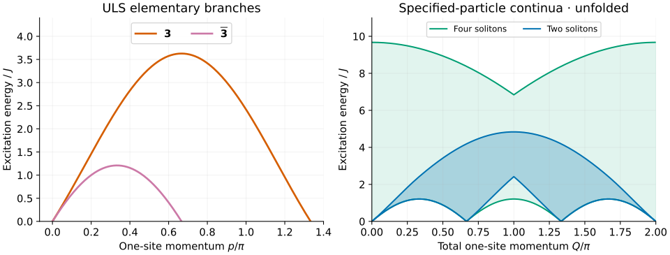
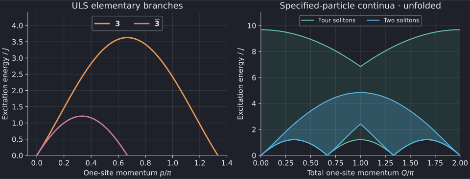
Full-size figure: light · dark.

Both elementary branches are gapless at their endpoints, with endpoint speed \(v=2\pi J/3\). Their maxima differ by a factor of three: approximately 3.627599 J for the 3 and 1.209200 J for the bar3. Do not interchange the momentum ranges when matching an SU(3) representation in your calculation.

There is also a global constraint. On a periodic fundamental chain with L divisible by three, the vacuum has zero SU(3) centre charge, or triality. A single 3 or bar3 has nonzero triality and is not an isolated state of that same balanced ring. A fractional/domain-wall ansatz can access elementary sectors that an ordinary local excitation above the singlet does not.

3. Why four particles matter¶

The smallest neutral pair decomposes as

The three physical spin operators and five quadrupoles form the adjoint 8. Acting on the singlet vacuum, they select adjoint states, not the singlet component of this pair. Under physical spin rotation, that adjoint contains spin 1 and spin 2.

The blue region is the kinematic interval for one 3 and one bar3. The green region is for two of each, which also allows adjoint channels. At total momentum Q=π the two-particle lower edge is approximately 2.418399 J, but the four-particle lower edge is only 1.209200 J. An adjoint MPS excitation below the blue edge is therefore not automatically a disagreement with Bethe ansatz: the two-particle edge is not the full sector threshold.

These are two specified particle contents, not an exhaustive enumeration of neutral states. Three equal representations can also be neutral, and larger particle numbers extend the spectrum. Neither plotted upper edge is a bound on the complete spectrum.

The shading is not intensity. Symmetry permits an observable to couple to a sector but does not guarantee nonzero weight at every momentum. In particular, the Q=0 summed SU(3) generators annihilate the singlet, even though the four-soliton kinematic interval has nonzero width there.

4. Compare a three-site unit cell¶

bethe-su3-dispersion --exchange 1 --points 193 --folded --csv su3-folded.csv

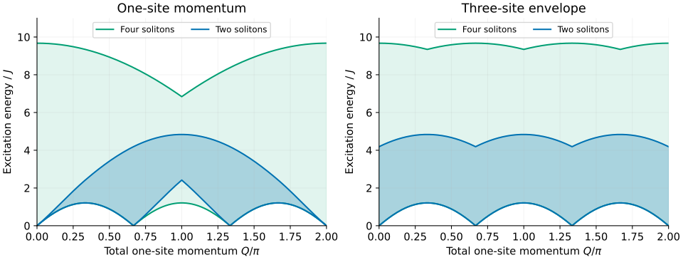
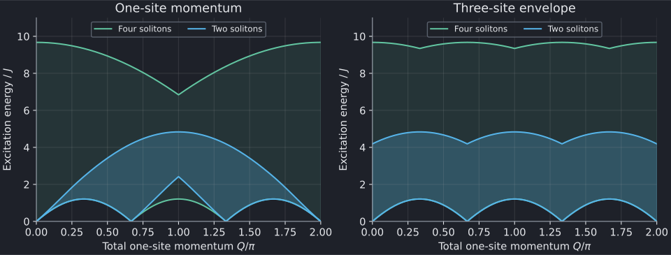
Full-size folding comparison: light · dark.

For a three-site cell the translation eigenphase is

The folded bounds take the envelope of Q, Q+2π/3 and Q+4π/3. The file keeps the original Q grid, so the right panel displays three repetitions over [0,2π]. For a plot against K/π, keep \(0\le Q/\pi\lt2/3\) and multiply that horizontal coordinate by three. The cell_momentum column supplies K directly.

--folded changes the continuum envelopes, not the elementary lines. The broad fundamental line is not made into a single-valued cell band by sorting its folded momentum. Keep distinct momentum images separate.

5. Reproduce the plots and check the comparison¶

Download unfolded and folded data. Each file has 193 rows per branch and includes provenance and convergence comments. The default fp64 arithmetic is sufficient for these figures; long-double and optional fp128 are also available in the frontend.

# From the source checkout:
python3 -m venv .venv
. .venv/bin/activate
python3 -m pip install -r docs/tutorials/requirements.txt
python3 scripts/plot_spin1_tutorial.py
# Regenerate both the ULS and TB examples using freshly built executables:
python3 scripts/plot_spin1_tutorial.py --bin-dir /path/to/bethe/bin
python3 scripts/plot_spin1_tutorial.py --check

The script plots actual exported values; its tests check representations, branch ranges, the unequal Q=π thresholds and three-image folding. Failed energies must not be replaced by zero. Empty cells in non-applicable columns—for example energy on a continuum row—are intentional.

Finite rings have discrete levels and finite-size corrections, not these continuous bands. Use the finite-ring solver for its supported ground states and the dispersion guide for formulas, normalization checks and finite-size comparisons. That guide explains the range convention used from Vörös–Penc and representation assignment from Doikou–Nepomechie.

Next: the spin-1 TB point, where elementary spinons carry spin 1/2 and quadrupolar response needs at least four of them.