Resolving the four-spinon contribution
Two-spinon thermodynamic spectrum · Selected-sector options
The two-spinon response is a useful starting point for an iMPS comparison, but it does not exhaust the local-spin spectrum. This tutorial adds four spinons at one interior spectral point and examines two different numerical questions: how well the quadrature resolves its chosen domain, and how much weight changes when that domain is extended.
We use the infinite spin-\(1/2\) XXX chain at zero temperature and field, \(H=J\sum_j\mathbf S_j\cdot\mathbf S_{j+1}\), with \(J=1\). The point is \(q=1.5\) radians/site and \(\omega=1.8J\). Output is the unbroadened longitudinal density \(S^{zz}(q,\omega)\); frequency integrals use \(d\omega/(2\pi)\).
Calculate both contributions
For this exact starting point and these controls, native long double passes
on the tested x86 system (64 significand bits), and is much faster than MPFR.
This is not a recommendation for every momentum or frequency: nearby points
can fail the same arithmetic screen. Check bethe-info on your platform;
long-double is a platform format, not a fixed bit count.
With a build or installation, run:
bethe-xxx-structure-factor-thermo --sectors 2,4 \
  --momentum 1.5 --omega 1.8 --precision long-double \
  --four-order 4 --four-cutoff 8 \
  --density-relative-tolerance 1e-6 --density-absolute-tolerance 1e-30 \
  --tolerance 1e-12 --threads 2 --csv point.csv --csv-table diagnostics=point-checks.csv
From a build directory, prefix the program with ./. The three output rows
are the two-spinon density, the four-spinon estimate and sum:2+4. They already
have compatible physical normalization: add the contributions directly.
The sum is still a partial response; six and higher sectors are absent.
This deliberately modest rule gives approximately
| Contribution | Density at this point |
|---|---|
| Two spinons | 0.8731304551 |
| Four spinons, order 4 and cutoff 8 | 0.1869408679 |
| Their partial sum | 1.0600713230 |
These extra digits identify the calculation, not its accuracy as an unrestricted four-spinon response. The refinement study below shows much larger integration changes than the arithmetic diagnostics.
Why does the calculation use two precisions?
The four-spinon integrand contains special functions and contour sums whose terms can nearly cancel. The selected floating-point format tells us how many digits we start with, but not how many survive that cancellation. The program therefore recomputes each form-factor density at two precisions and checks their agreement before using it in the quadrature.
You select one format with --precision; the program chooses the lower
comparison automatically. For the command above on the tested x86 system,
it evaluates the same spinon configuration in double (53 significand bits)
and long double (64 significand bits). Each calculation starts from the same
geometry coordinates, converted separately into its arithmetic format. The
lower result is a fresh evaluation, not a rounded copy of the higher one.
The higher precision is called the guard precision in the diagnostics.
Increasing precision checks sensitivity to roundoff. Increasing the number of contour terms checks a different source of error: truncating the form-factor representation. The default controls combine both comparisons:
| Contour controls | Lower-precision evaluation | Higher-precision evaluation |
|---|---|---|
| 64 residue terms, tail order 16 | double, 53 bits |
long double, 64 bits |
| 80 residue terms, tail order 20 | double, 53 bits |
long double, 64 bits |
Both rows must pass the arithmetic and contour checks, and their higher-precision results must agree within the estimated allowances. The program keeps the higher-precision result from the larger contour budget; the four values are not averaged. This happens at each quadrature node, rather than by integrating the whole spectrum twice. The six-spinon calculation uses the same check at its sampled configurations.
These are numerical stability checks, not rigorous error bounds. In particular, they do not measure the outer quadrature error or the weight excluded by the soft cutoff. A failed precision comparison can also be caused by the lower calculation even when the higher result is accurate.
When changing the point or integration controls, inspect the exit status and
diagnostics again. If the arithmetic screen fails, retain the failure and repeat
the whole query with --precision fp128 where available. With intermediate
native long double, this strengthens the density pair from 53/64 to 64/113
bits. If the complete query still fails, try MPFR with --precision bits-128
and then more bits as needed. A failed screen does not supply an approximate spectral
value or a usable partial sum.
The starting command uses a \(10^{-6}\) relative density screen, comfortably below the order/domain changes demonstrated here. Wider-reference checks at contrasting points support that choice; they do not certify a whole spectral curve. Even at this tolerance, some ordinary points need a stronger pair. See the neighbourhood study before extending the command to a grid.
Change order and soft cutoff separately
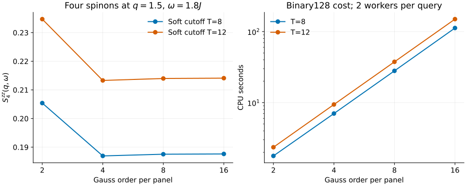
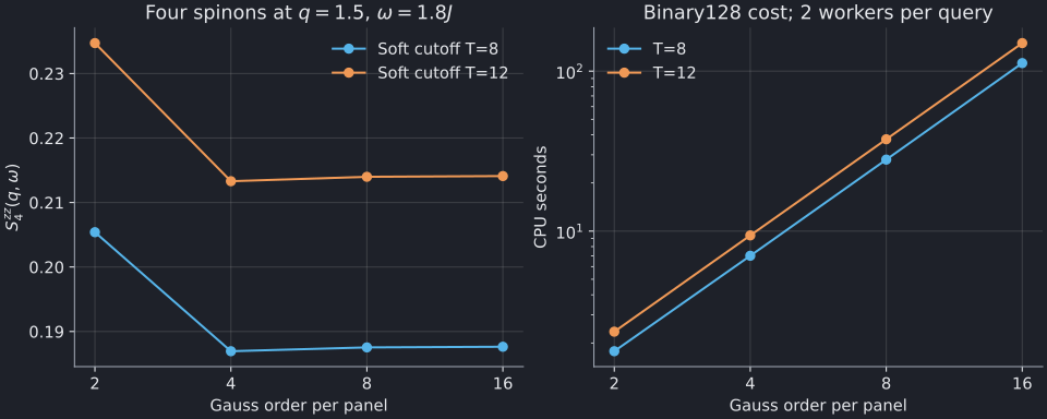
Each curve holds the soft cutoff fixed and increases the Gauss order per panel. Comparing points vertically at the same order changes the integration domain instead. The two-spinon baseline is unchanged throughout this study. The plotted costs use binary128 with a native 64/113-bit density pair and two workers per query. They are separate from the cheaper native 80-bit starting example and the wider MPFR reference calculations below.
--four-cutoff T is a log-radius cutoff in the support-adapted four-spinon
coordinates. Increasing it includes configurations closer to a soft endpoint.
It is not a cutoff on frequency, a number of spinons, or a bound on every
absolute rapidity. See the integration geometry
for its definition.
The higher-order points can stabilize within one curve while the curves remain separated. That is convergence within a truncated domain, not evidence that the soft contribution has been exhausted. At order 16, changing the cutoff from 8 to 12 changes the four-spinon density by about 0.02647; changing the order from 8 to 16 at cutoff 12 changes it by about 0.00011. A small order change alone would therefore give a misleading accuracy impression here.
The frontend can make four comparisons in one command. Finer orders introduce
more difficult nodes: at the refinement study's stricter \(10^{-8}\) relative
tolerance, orders 8 and 16 fail the native 53/64-bit density screen at both
cutoffs. Keep those failures; do not use an
incomplete prefix. For the validated refinement study, replace --precision
long-double with --precision fp128 and replace the starting command's
--density-relative-tolerance 1e-6 with --density-relative-tolerance 1e-8.
Then add these two refinement options:
--four-refine-order 8 --four-extended-cutoff 12
It evaluates coarse/fine orders on both domains. The displayed four-spinon
value uses the fine order on the extended domain. quadrature_difference
and cutoff_change report separate comparisons; neither is an automatic
estimate or correction of the remaining tail. Check the individual diagnostic
columns as well as the density and its status.
Arithmetic accuracy is a different check
For each precision pair, the difference between the density values, the kernels' roundoff indicators and the change in the scalar prefactor form the arithmetic diagnostic. This diagnostic plus the estimated contour remainder must fit within \(\mathrm{atol}+\mathrm{rtol}\,|W_{\mathrm{high}}|\), where \(W_{\mathrm{high}}\) is the higher-precision form-factor density at that configuration. The tolerance applies to this inner calculation, not directly to the final spectrum. The precision guide lists the actual native pairs, portable selection and separate MPFR geometry and density controls.
A fixed-control comparison of the starting point, using the stricter \(10^{-8}\) relative density screen, gives:
| Arithmetic | Density comparison / guard bits | Result | CPU seconds |
|---|---|---|---|
| Binary64 | 24 / 53 | Arithmetic screen fails | 0.0069 to failure |
| x86 long double | 53 / 64 | Complete | 0.329 |
| Binary128 | 64 / 113 | Complete | 6.86 |
| MPFR, 128 bits | 64 / 128 | Complete | 51.0 |
| MPFR, 192 bits | 128 / 192 | Complete | 65.1 |
The complete native result agrees with MPFR192 to about \(1.14\times10^{-16}\) relative; MPFR128 and MPFR192 agree to about \(2.42\times10^{-38}\). That is much more arithmetic agreement than this demonstration needs. It does not resolve the large omitted soft contribution. The native arithmetic screening diagnostic is about \(4.8\times10^{-11}\) here, also well below the observed order/domain changes. Agreement between wider runs is a separate check.
Every row uses the same quadrature, domain, 64/80 contour terms, 16/20 tail orders, density tolerances and explicit two-spinon tolerance of \(10^{-12}\). One worker is used for this comparison. The compact record retains the failed binary64 contribution and its missing partial sum, as well as successful values, diagnostics, controls, source revisions and costs. Check or regenerate all five formats with:
python3 scripts/check_xxx_four_spinon_precision.py --check
# Requires a build with binary128 and MPFR; retains expected failures:
python3 scripts/check_xxx_four_spinon_precision.py \
--solver bethe-xxx-structure-factor-thermo --raw-dir precision-exports
The failed native higher-order checks do not prove the 64-bit-significand answer would be wrong: its 53-bit comparison may be limiting. They do mean that this pair cannot certify every node under the requested policy. Increasing the precision pair and repeating the complete calculation tests that issue; loosening the guard solely to obtain success does not.
Changing the point can change the precision requirement
An independent follow-up tests 54 points: six momenta from 0.6 to 3 radians and nine frequencies from \(1J\) to \(4.5J\), all at order 4 and cutoff 8. Five lie outside support. Among the remaining 49:
| Arithmetic | rtol=1e-8 |
rtol=1e-6 |
rtol=1e-4 |
|---|---|---|---|
| Binary64, 24/53-bit pair | 0 complete | 0 complete | 0 complete |
| x86 long double, 53/64-bit pair | 26 complete | 47 complete | 49 complete |
| Binary128, 64/113-bit pair | 48 complete | 49 complete | Not measured |
The two long-double failures remaining at \(10^{-6}\) are \((q,\omega/J)=(2.5,1.8)\) and \((1.5,4.5)\). MPFR128 completes both at the stricter \(10^{-8}\) tolerance, as well as \((1.5,3)\), where native arithmetic passes at \(10^{-6}\) but fails at \(10^{-8}\). The successful long-double values at these three points differ from their MPFR128 references by less than \(1.3\times10^{-16}\) relative. MPFR192 independently confirms the first reference. The recorded binary128 failure used the earlier 53-bit lower comparison; the original audit predates the stronger native pair.
The binary128 row comes from a later 98-query follow-up using the intermediate native comparison. At \(10^{-8}\), the only remaining failure is \((q,\omega/J)=(1.5,4.5)\); at \(10^{-6}\) all 49 supported points complete. Every completed S4 estimate agrees with its matched MPFR128 reference within \(1.3\times10^{-30}\) relative. Thus binary128 is a useful retry before MPFR, but the strict screen still does not pass everywhere on this grid. The original failed point is retained. Both comparisons concern the same finite quadrature and do not establish its physical accuracy.
These results distinguish screen coverage from measured value accuracy. The original binary64/long-double grid costs 17.5 CPU seconds; five wider-reference checks cost 81.8 CPU seconds on the same i7-12700KF. These timings select only sector 4; do not compare them directly with the two-sector timings above. Wider values were checked at three contrasting points for long double; the later binary128 study checks every completed value. Its costs are recorded separately on a Xeon Gold 6254 with two workers per query. Passing all long-double points at \(10^{-4}\) is therefore not a blanket accuracy recommendation. Choose a tolerance from the observable's error budget, compare against stricter wider references, and keep that choice separate from order and domain checks.
Check the retained binary128 coverage and value comparisons without running the solver:
python3 scripts/check_xxx_four_spinon_native_neighbourhood.py
The compact record retains all 329 outcomes, effective precision, diagnostics, costs and raw hashes. Check it or repeat the study, including expected numerical failures, with:
python3 scripts/check_xxx_four_spinon_neighbourhood.py --check
python3 scripts/check_xxx_four_spinon_neighbourhood.py \
--solver bethe-xxx-structure-factor-thermo --raw-dir neighbourhood-exports
With the intermediate native comparison, binary128 completes all eight order/cutoff points and agrees with the MPFR192 S4 references within \(6.3\times10^{-31}\) relative. The complete binary128 grid costs about 5.80 CPU minutes, compared with 41.0 CPU minutes for the earlier MPFR128 reference study on the same shared Intel Core i7-12700KF, with two workers per query. This is why binary128 is the next arithmetic choice after native 80-bit.
The new native record retains all eight complete quadratures. The earlier refinement record retains the failed 53/113-bit binary128 comparisons and the MPFR128/192 references. Those failures were a limitation of the old lower comparison; they were not evidence that the binary128 value was inaccurate. Both records keep the same strict tolerances and contour controls. Neither determines the remaining soft-tail contribution.
The density screen is \(\mathrm{atol}+\mathrm{rtol}|W|\). Its relative
term dominates above \(|W|=10^{-22}\) in the strict \(10^{-8}\) comparison,
or \(10^{-24}\) in the starting command's \(10^{-6}\) comparison.
The 1e-30 absolute tolerance is a near-zero floor,
not a demand for thirty-digit relative accuracy. The accuracy guide
explains the scale and the separate solver, contour, quadrature, sampling and
tail checks. For a small example of actual information loss and a stable
reformulation, see the one-magnon precision tutorial.
Cost and practical scope
The strict native precision-check point takes about 0.33 CPU seconds on the measured Intel Core i7-12700KF. The binary128 refinement grid above takes about 5.80 CPU minutes in total with two workers. Its order-4/cutoff-8 point uses about 3.6 seconds wall and 7.0 CPU seconds; the largest point, order 16 and cutoff 12, uses about 75 seconds wall and 150 CPU seconds. The original MPFR192 grid took about 54 CPU minutes and remains an optional arithmetic reference. These shared-host measurements describe the recorded runs, not portable performance guarantees.
Doubling order increases the number of nodes in both integration directions. Start with a few representative points and separate the order and domain checks before requesting a dense spectral grid. More scheduler workers help with independent node evaluations; they do not replace numerical refinement.
For integrated intensity or the first frequency moment, use
bethe-xxx-moments-thermo. It evaluates the moment
measure directly rather than integrating a plotted frequency grid. Its
fixed-momentum and global four-spinon domains have different cutoff controls;
copying the number 8 from this example does not copy the physical domain.
Try a small six-spinon slice
The same program can evaluate six spinons using independent sampling replicates. This is a small execution and reporting example, at a different momentum from the four-spinon study above:
bethe-xxx-structure-factor-thermo --sectors 6 \
--momentum 1.57079632679489661923132169163975 \
--omega-min 1.8 --omega-max 2.2 --points 3 \
--precision long-double --six-cutoff 8 --replicates 4 --samples 32 \
--seed 42 --threads 2 --density-relative-tolerance 1e-5 \
--diagnostics --replicate-output --quiet --json slice.json
A fresh run of the installed program gave:
| \(\omega/J\) | Six-spinon density | Sampling standard error |
|---|---|---|
| 1.8 | 0.00003123 | 0.00002380 |
| 2.0 | 0.00018661 | 0.00012265 |
| 2.2 | 0.00017248 | 0.00011482 |
These errors are 66–76% of the estimates. Four replicates do not establish
reliable confidence intervals, and the absolute-rapidity cutoff 8 also omits
substantial soft weight. The table demonstrates fresh calculation and separate
error reporting; it is not a resolved six-spinon curve. More samples address
sampling variation, while a larger cutoff addresses a different omission.
The two cutoff types must not be equated: --six-cutoff bounds absolute
rapidities, whereas --four-cutoff bounds the soft log-radius coordinate.
The native run used 0.31 seconds wall time and 0.38 CPU seconds on the same CPU model, with two workers. Its means agree with the 384-bit reference to within \(2.7\times10^{-16}\) relative. The eight-format comparison retains controls, source revisions, timings and failed formats; the replicate exports allowed independent reconstruction of the means and sampling errors. Binary64 fails both arithmetic and exponent-range checks on this stream; the updated binary128 64/113-bit pair completes in 7.32 CPU seconds, while the successful MPFR128 alternative costs about 44 CPU seconds. These results justify the native setting for this small example, not for a new seed or a larger soft domain. See six-spinon sampling before extending it.
Changing the seed can expose a failed density screen even at this small cutoff. An independent scan of seeds 1–40 retained every outcome: seeds 2 and 35 fail in native 80-bit arithmetic at the printed \(10^{-5}\) tolerance. Repeating both whole queries in binary128 with the 64/113-bit pair completes without changing the tolerance, domain or streams. Across seeds 42, 2 and 35, the means, sampling errors, replicate means and maxima agree with MPFR192 within \(4.9\times10^{-30}\) relative. The native follow-up retains complete replicate summaries and source identities; each query took 6.3–7.4 CPU seconds. These checks do not establish success for every seed or larger sample count.
For a small precision exercise, replace --seed 42 with --seed 2, retain the
native 80-bit failure, then try --precision fp128 where available. The
effective comparison pair is reported in the output. MPFR128 and MPFR192 also
complete the same query at the original tolerance, with the three means
agreeing within \(4.4\times10^{-37}\) relative. Use those optional wider
replays to check arithmetic separately from sampling and the omitted domain.
Native arithmetic with a \(10^{-3}\) density tolerance also completes seed 2; its means agree with the strict MPFR192 reference within \(3.3\times10^{-16}\). That comparison supports a cheaper inner accuracy budget for this particular demonstration. It is not permission to keep loosening a screen until an unknown query passes. Binary64 still fails, including an exponent-range failure. The seed comparison retains the 40 discovery outcomes, four replays, sampling diagnostics, matched stream/count checks and costs. The strict MPFR128/192 replays cost 37.8/48.5 CPU seconds; the looser native replay costs 0.31. Sampling errors remain large. Never search for a passing seed or discard failed observations to obtain a plotted estimate.
To include lower sectors at these same spectral points, use --sectors 2,4,6
and refine their numerical controls separately. No normalization step is needed.
Reproduce and extend the study
The checked compact data retain all eight finite-domain estimates, separate diagnostics, work counts, timings, compiler/hardware information and exact Bethe/Uni20 source revisions. With NumPy and Matplotlib available, reproduce both light and dark figures:
python3 scripts/plot_xxx_four_spinon_tutorial.py
To recalculate the points from fresh inputs, put the program on PATH:
python3 scripts/plot_xxx_four_spinon_tutorial.py \
  --solver bethe-xxx-structure-factor-thermo --threads 2 \
  --raw-dir four-spinon-exports
Use a new raw-output directory; existing exports are not overwritten. This
runs all eight calculations and can take tens of minutes. The script validates
controls, statuses, provenance, the two-spinon reference and physical partial
sums before replacing the compact dataset or drawing a figure. No target
four-spinon fraction is inserted. Literature is available through
--references and CITATIONS.md.