Hubbard spinons, holons and energy conventions
An infinite, half-filled Hubbard chain is a useful reference for an iMPS excitation calculation: its spin excitations are gapless, while its charge excitations are gapped. This tutorial plots the elementary lines at \(U/t=4\), then shows exactly how the energies change between interaction conventions. A second tutorial moves away from half filling.
The figures and CSVs are included. To generate your own, build
bethe-hubbard-dispersion; no Python is needed to run the solver. The commands
below assume the executable is on PATH; see running the programs.
All calculations here use default fp64.
1. Choose a Hamiltonian
We set hopping \(t=1\), density \(n=N/L=1\), zero field and zero temperature. The default interaction is symmetric:
This is the SO(4)-symmetric convention. The unshifted convention instead uses \(U n_{j,\uparrow}n_{j,\downarrow}\). They differ by a particle-number term and a constant, so their eigenstates agree but charge-changing excitation energies do not. We will keep that distinction visible in the plots.
2. Export the elementary lines
bethe-hubbard-dispersion --u 4 --density 1 --points 129 \
  --convention symmetric --reference hamiltonian --csv hubbard-half-symmetric.csv
The default --branch all writes three families into the dispersion table:
| Branch | Particle change \(\Delta N\) | Spin | Exported momentum \(p/\pi\) |
|---|---|---|---|
spinon |
0 | 1/2 | [0, 1] |
holon |
−1 | 0 | [−1, 1] |
antiholon |
+1 | 0 | [−1, 1] |
Use p_over_pi on the horizontal axis and energy on the vertical axis.
The grid is uniform in physical dressed momentum, not the Bethe parameter.
Each branch has 129 points, including endpoints. The charge endpoints −π
and π represent the same Brillouin-zone point.
Full-size figure: light · dark.
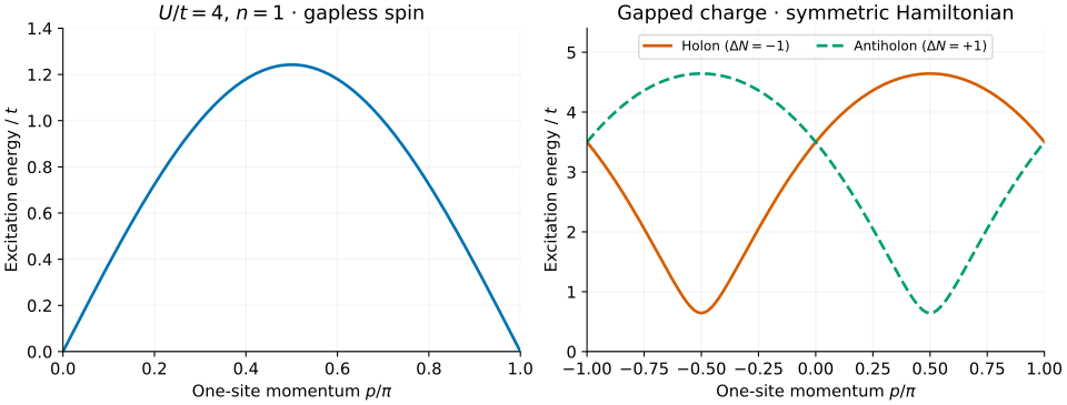
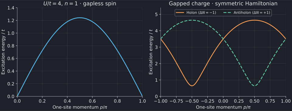
The spinon energy vanishes at both ends and reaches about 1.242281 t at \(p=\pi/2\). The charge branches have the same minimum, 0.643364 t, at \(p=-\pi/2\) for the holon and \(p=+\pi/2\) for the antiholon. Their momenta at equal bare charge parameter differ by π modulo 2π.
Do not confuse a single-charge minimum with the full charge gap:
Here each symmetric charge minimum is \(\Delta_c/2\). The value of \(\Delta_c\) is unchanged by switching interaction convention.
3. Understand the energy shifts
At fixed number of sites, the two Hamiltonians and their excitation energies obey
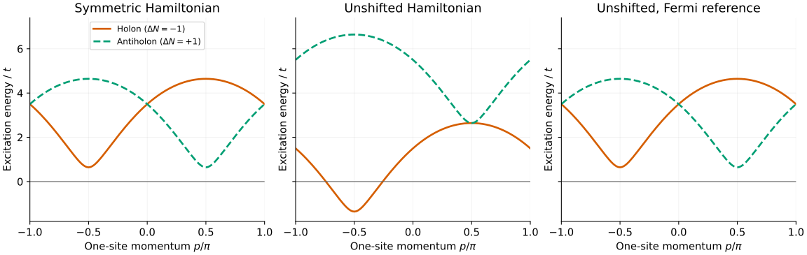
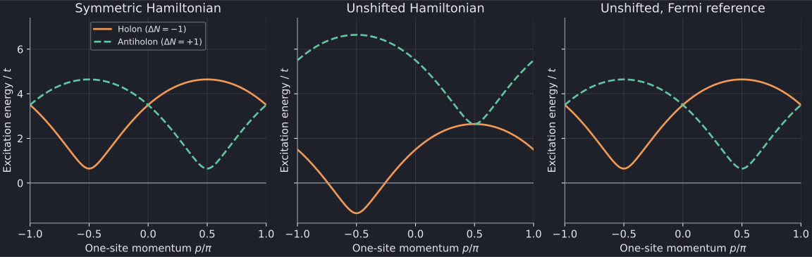
For U=4, the spinon is unchanged, the holon shifts down by 2, and the antiholon shifts up by 2. Export the second convention and a chemical-potential-subtracted version:
bethe-hubbard-dispersion --u 4 --points 129 \
  --convention unshifted --reference hamiltonian --csv hubbard-half-unshifted.csv
bethe-hubbard-dispersion --u 4 --points 129 \
  --convention unshifted --reference fermi --csv hubbard-half-fermi.csv
Full-size comparison: light · dark.
A negative unshifted holon energy is not a numerical failure or evidence that the fixed-density ground state is unstable. Removing an electron also removes its chemical-potential contribution. For a comparison with an MPS calculation of \(H-\mu N\), use
At half filling, the tool chooses the middle of the Mott plateau:
\(\mu_{\mathrm{sym}}=0\) and \(\mu_{\mathrm{unshifted}}=U/2\). Consequently,
the first and third panels coincide, with a nonzero charge gap remaining.
The columns symmetric_energy and fermi_energy keep their respective meanings
regardless of the choice for energy.
4. Compare with an excitation ansatz
These are fractional elementary excitations, not isolated electron levels on a finite ring. A single spinon or holon needs a compatible domain-wall/topological excitation sector. A local electron changes both charge and spin; its spectral function is not simply one of these curves.
For a useful comparison:
- Match hopping, U, particle change and spin before aligning curves.
- Match the Hamiltonian convention and whether μ has been subtracted.
- Match the momentum origin of the domain-wall construction. Enlarged cells fold one-site momenta; there is no universal additional gauge shift.
- Treat these as elementary lines, not guaranteed lowest energies in every sector. Multiparticle states can lie below an elementary line at the same total momentum. No intensity or spectral weight is plotted.
For neutral pairs, the separate Hubbard continuum tool provides half-filled two-spinon bounds.
An elementary line inside a continuum
Osborne–McCulloch, Secs. III D and IV B and Fig. 5, demonstrates this distinction at U=5t, half filling, with the symmetric interaction. A chargon can overlap a chargon–two-spinon continuum in the same charge and spin-projection sector. Energy minimization then favours lower continuum states, not the elementary chargon.
Instead, the paper follows the chargon by minimizing its excitation energy variance, using the previous momentum's optimized state to initialize the next. For a normalized finite-system state, the underlying diagnostic is
The infinite-MPS construction isolates the excitation contribution from the background; do not directly subtract two divergent extensive expectations. Small variance tests eigenstate quality, not whether an energy is the sector minimum. Branch continuity and quantum numbers remain important.
To obtain Bethe reference lines at the paper's coupling:
bethe-hubbard-dispersion --u 5 --density 1 --points 129 \
  --convention symmetric --reference hamiltonian --csv hubbard-u5.csv
Align the domain-wall momentum origin and unit-cell convention before comparing
with Fig. 5; its quoted crossing momentum is not automatically our p.
This command supplies elementary energies, not MPS variances or the
three-particle continuum. The figures above remain U=4 examples, not a
reproduction of the paper's numerical MPS data.
5. Reproduce and check
Download the exports: symmetric Hamiltonian, unshifted Hamiltonian, and unshifted with Fermi reference.
From the source checkout:
python3 -m venv .venv
. .venv/bin/activate
python3 -m pip install -r docs/tutorials/requirements.txt
python3 scripts/plot_hubbard_tutorial.py
# Optional: regenerate the data for both Hubbard tutorials before plotting.
python3 scripts/plot_hubbard_tutorial.py \
  --solver bethe-hubbard-dispersion
The script uses exported columns for
every curve. It rejects failed runs, missing/non-finite energies, incomplete
momentum grids and unexpected conventions. Infinite spin rapidities at
the gapless endpoints are valid; infinite energies are not. Preserve the
leading and trailing # comments, which record provenance and run success.
--check validates the saved data without importing Matplotlib.
The dispersion guide explains error estimates,
precision controls and numerical limits. The half-filled formulas are recorded
in Essler–Korepin; their interaction
parameter is our U/4. Run bethe-hubbard-dispersion --references for the full
tool bibliography.
Next: dope the chain and follow its gapless charge branches.