Non-Hermitian XXZ: energies are not enough¶

All tutorials · Model guide · Potts tutorial

A real list of energies does not make a Hamiltonian Hermitian. This example first solves a restricted real-root family with imaginary boundary fields, then visits an exactly enumerated endpoint where some equal eigenvalues belong to Jordan blocks, not independent eigenvectors.

1. Keep the imaginary end fields¶

With spin-half operators and J=1, the open-chain Hamiltonian is

\[ H=\sum_{j=1}^{N-1}\left(S_j^xS_{j+1}^x+S_j^yS_{j+1}^y+ \Delta S_j^zS_{j+1}^z\right) +\frac{i\sqrt{1-\Delta^2}}2(S_1^z-S_N^z). \]

This is not the Hermitian free-end XXZ chain. Omitting the imaginary fields changes the problem. There is no translation momentum on this open chain. The source normalization is one quarter of the Pauli Hamiltonian in Gainutdinov et al., with the boundary sign reversed; spatial reflection reverses that sign without changing the energies.

For a small regular-root scan, choose N=8, Δ=0.6 and four through-lines:

bethe-xxz-qg-obc 8 --delta 0.6 --through-lines 4 --excitations all \
  --csv-table levels=qg-levels.csv --csv-table reference=qg-sea.csv \
  --csv-table roots=qg-roots.csv

Here \(\ell=N-2M=4\) means M=2 Bethe roots and the representative has \(S^z=\ell/2=2\). Through-lines label the Temperley–Lieb sector, not ordinary SU(2) spin or a promised root-of-unity degeneracy. The allowed finite-real window has five slots, so this scan returns \(\binom52=10\) levels. The full fixed-\(S^z\) spin space has dimension \(\binom82=28\).

The sea energy is approximately -1.74502170 and the first returned gap is 0.35518911. gap_from_sea subtracts the selected consecutive-label sea, not an independently established global ground state. all exhausts this regular window only; it does not supply missing complex roots or descendants. The model guide explains failed-candidate accounting and the bounded scan.

2. At Δ=0, switch from Bethe roots to Jordan blocks¶

The endpoint has a separate exact construction:

bethe-xxz-qg-obc 6 --delta 0 --sz 0 --csv-table blocks=qg-blocks.csv

It lists the complete fixed-magnetization Hamiltonian spectrum and block sizes. The regular --through-lines, --excitations and --roots options do not apply here. --sz keeps its sign; it is not folded to an absolute value.

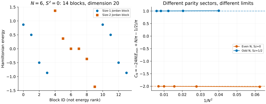
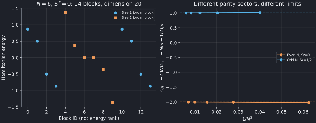
Fourteen Hamiltonian Jordan blocks at N=6 occupy a twenty-dimensional sector; even and odd chains have distinct Casimir limits.

The left panel has 14 rows but a sector dimension of 20: eight size-one blocks and six size-two blocks. Each square denotes one eigenvector plus one generalized eigenvector, not two ordinary eigenvectors. Coincident energies in different rows must not be merged. Block ID is an enumeration label, not an energy rank or a momentum.

The simplest example is N=2, \(S^z=0\). In the ordered basis \(|\downarrow\uparrow\rangle,|\uparrow\downarrow\rangle\),

\[ H=\frac12\begin{pmatrix}-i&1\\{}1&i\end{pmatrix},\qquad H\ne0,\qquad H^2=0. \]

There are two algebraic zero eigenvalues, but only one eigenvector. If \(Hw=0\) and \(Hv=w\), then \(e^{-itH}v=v-itw\): the generalized vector produces a polynomial time factor invisible in an energy list. This is not unitary dynamics. The frontend gives block sizes, not the spin-basis vectors w and v.

For numerical comparisons use a general complex eigensolver, never a self-adjoint solver. Near a defective eigenvalue, tiny numerical perturbations can split the reported eigenvalues. The optional check below compares nullities of \(H-E\), \((H-E)^2\) and \((H-E)^3\), rather than trying to infer Jordan structure from tiny eigenvalue separations.

3. Count the sector before interpreting its spectrum¶

The endpoint maps to fermions with one-particle energies \(\cos(\pi k/N)\), k=1,…,N-1, and an additional zero mode. For even N, k=N/2 collides with that extra zero and forms a size-two block.

For each subset of nonzero modes, let z denote zero-space occupation:

Chain	Allowed z	Block size
Odd N	0 or 1	1
Even N	0 or 2	1
Even N	1	2

The number of down spins is the number of occupied nonzero modes plus z. The block energy is the sum of their cosines. Summing block sizes, rather than counting rows or distinct energies, must give \(\binom NM\). The odd/even diagonalizability distinction agrees with Gainutdinov et al., Appendix D.

For N=7, \(S^z=1/2\), all 35 blocks have size one. At N=6, \(S^z=\pm1\), the two signed sectors have equal spectra; the fully polarized sectors each contain a single zero-energy block. These cases are included in the downloads. Endpoint enumeration is bounded by --max-blocks and --max-mode-entries; budget refusal is an error, not a partially complete spectrum.

4. A negative Casimir coefficient needs a sector label¶

The right panel uses the minimum energy from each exported sector, with even N at \(S^z=0\) and odd N at \(S^z=1/2\). They obey the finite sums

\[ \begin{aligned} E_{\min}^{\mathrm{even}}&=\frac{1-\cot(\pi/(2N))}{2} =-\frac N\pi+\frac12+\frac{\pi}{12N}+O(N^{-3}),\\{} E_{\min}^{\mathrm{odd}}&=\frac{1-\csc(\pi/(2N))}{2} =-\frac N\pi+\frac12-\frac{\pi}{24N}+O(N^{-3}). \end{aligned} \]

Subtracting the bulk and boundary terms defines

\[ C_N=-\frac{24N}{\pi}\left(E_{\min}+\frac N\pi-\frac12\right). \]

The even sequence approaches -2, the odd sequence +1. At N=12 and 13 the values are -2.00228837 and 1.00170596. Both come from the same boundary Hamiltonian; combining parities into one fit would be misleading.

In a boundary-CFT interpretation with velocity one, this coefficient measures \(c_{\mathrm{eff}}=c-24h_{\min}\), not c without identifying the boundary sector and its lowest conformal weight. The open-chain factor 24 also differs from the periodic factor 6 in the Potts example. This plot is a checked finite-size diagnostic, not a determination of all conformal towers or a replacement for root-of-unity representation theory.

For non-Hermitian MPS work, energies and right-state residuals are only part of validation. Left/right eigenvectors, their normalization and generalized eigenvectors can matter for observables; this energy frontend does not supply them. A small residual alone cannot certify a well-conditioned eigenbasis.

5. Reproduce and validate¶

Regular scans at N=8, Δ=0.6:

Through-lines	Ranked levels	Sea reference	Joined roots
4 (two roots)	CSV	CSV	CSV
6 (one root)	CSV	CSV	CSV

Complete endpoint sectors:

Sequence	`blocks` exports
Even N, Sz=0	2, 4, 6, 8, 10, 12
Odd N, Sz=1/2	5, 7, 9, 11, 13
N=6 signed sectors	Sz=+1, Sz=-1, Sz=+3, Sz=-3

With the plotting dependencies, from the source checkout:

python3 scripts/plot_potts_qg_tutorial.py --check
python3 scripts/plot_potts_qg_tutorial.py
# Optional: regenerate both this and the Potts tutorial.
python3 scripts/plot_potts_qg_tutorial.py --solver-dir /path/to/bethe/bin
# Optional independent matrix checks; requires NumPy.
python3 scripts/plot_potts_qg_tutorial.py --check --oracle
python3 -m unittest discover -s scripts -p 'test_tutorial_potts_qg.py'

The script validates regular roots in both logarithmic and complex equations, joins them to ranked states and checks every endpoint mode subset and sector dimension. The optional oracle checks spin matrices through N=7, including Jordan nullities, and both regular N=8 scans. Regression tests also reject missing blocks, incorrect sizes, wrong joins and failed metadata. These fp64 examples can be repeated in native long-double or optional fp128; extra precision does not turn a defective Hamiltonian into a diagonalizable one.