XXX: when a converged energy is not accurate enough¶

View this page on GitHub

Most of the finite-chain tutorial works well in binary64. When is extra precision actually useful? A long-wavelength one-magnon state gives a particularly clear test: the Bethe equation can have a computed residual of zero while rounding has erased its entire energy shift.

We can check this independently against an exact dispersion. Even the enormous ring lengths below are inexpensive: there is one root, not a half-filled sea of N/2 roots. These are deliberately demanding conditioning tests, not suggested sizes for antiferromagnetic ground-state calculations.

1. A small energy on top of a large reference¶

Use the usual periodic Hamiltonian and the fully polarized state:

\[ H=\sum_j\mathbf S_j\cdot\mathbf S_{j+1},\qquad E_{\mathrm F}=N/4. \]

One flipped spin with momentum \(p=2\pi/N\) has

\[ E(p)=N/4-\delta_N,\qquad \delta_N=1-\cos p=2\sin^2(\pi/N). \]

Here \(\delta_N\) is the positive energy lowering from the polarized state, not an excitation gap above the antiferromagnetic singlet. Equivalently, it is the positive one-magnon excitation energy for the ferromagnetic Hamiltonian \(-H\). Its quadratic small-momentum dispersion is the familiar ferromagnetic spin wave.

For one root, the logarithmic Bethe equation and its solution are

\[ N\arctan z=\pi I,\qquad I=N/2-1,\qquad z=\cot(\pi/N),\qquad \delta_N=\frac{2}{1+z^2}. \]

The exported rapidity is \(z=2\lambda_{\mathrm{ABA}}\). The integer I labels the state; the rapidity is a continuous coordinate. As N grows, this particular state approaches an infinite rapidity, but remains finite for every run here.

2. Reproduce the loss of a physical energy scale¶

With an arbitrary-precision build, run the same state in two precisions:

bethe-xxx-pbc 1000000 --quantum-numbers 499999 --precision fp64 \
  --roots --format json > magnon-fp64.json
bethe-xxx-pbc 1000000 --quantum-numbers 499999 --precision bits-256 \
  --roots --format json > magnon-bits256.json

This root-only calculation needs Uni20's arbitrary-precision scalar support, but not MPLAPACK matrix kernels. bethe-info reports the capabilities of your build. --precision digits-100 is another valid request; it selects 333 significand bits. It is not an output-format setting.

At this size, the true energy lowering is approximately \(1.9739208802113778\times10^{-11}\), subtracted from 250,000. In the saved binary64 run the exported total energy is 249999.99999999997. Subtracting that decimal export from 250,000 gives \(3\times10^{-11}\): about 52% relative error in the energy lowering, despite a computed residual of zero. The 256-bit export retains the shift to better than 60 relative decimal digits. Exact last digits depend on the compiler and math library.

Do the subtraction without silently rounding the export back to binary64:

import json
from decimal import Decimal, localcontext

for filename in ("magnon-fp64.json", "magnon-bits256.json"):
    with open(filename) as stream:
        table = json.load(stream)["tables"]["states"]
    row = dict(zip((c["id"] for c in table["columns"]), table["rows"][0]))
    cell = row["energy"]
    # Runtime-precision cells carry both a decimal string and a precision tag.
    text = cell["value"] if isinstance(cell, dict) else cell
    with localcontext() as context:
        context.prec = 110
        shift = Decimal(table["metadata"]["Sites"])/4 - Decimal(text)
        print(filename, shift)

Using float(text) first would discard the additional information. Increasing the number of printed digits after a binary64 solve cannot recover it either.

3. Better formulas and more precision solve different problems¶

Relative error in the one-magnon energy lowering, obtained either from total energy or directly from the exported root, across five working precisions

Download the numerical exports and provenance.

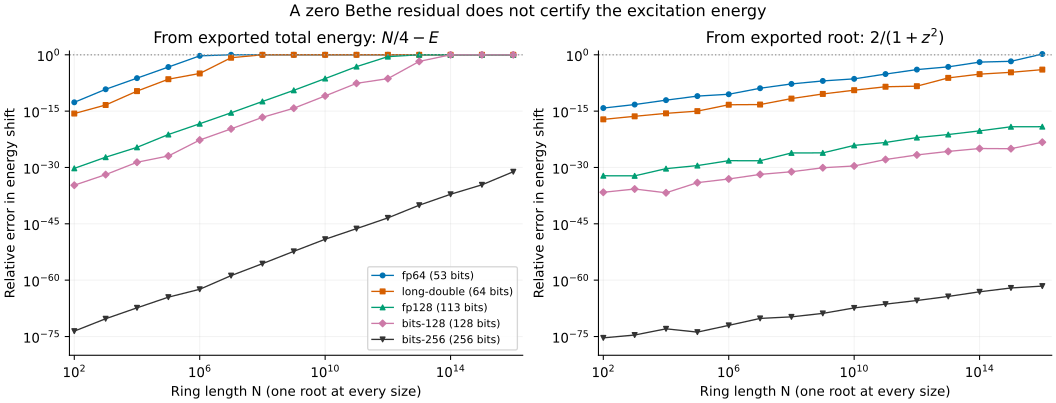
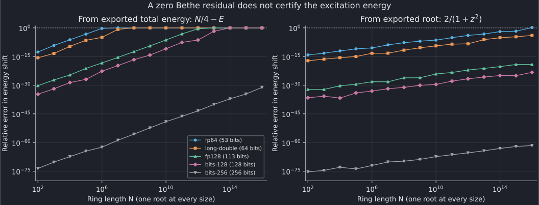
The left panel uses \(N/4-E\). The right panel instead uses \(2/(1+z^2)\), with the root from the same solve. Both are evaluated in 110-digit decimal arithmetic after reading the exports, and compared with an independent evaluation of \(2\sin^2(\pi/N)\). Thus the curves measure the information retained by the solver and its decimal export, not an accidental binary64 conversion in the plotting script. Only the final error coordinates are converted to ordinary plotting numbers.

The saved long-double runs use x86 80-bit extended precision, with 64 significand bits. fp128 has 113 significand bits; bits-128 has 128. On other platforms, long-double may mean something different—check bethe-info.

Subtracting extensive energies loses digits. The total energy scales as N while this shift scales as \(N^{-2}\). The ratio of scales is approximately \(N^3/(8\pi^2)\), so subtracting the total energies loses roughly three extra decimal digits for each factor of ten in N. At \(N=10^{12}\), even the binary128 export has about 32% relative error in the shift. At \(N=10^{16}\), binary128 and bits-128 lose it completely; bits-256 still resolves it with relative error below \(10^{-30}\).

A stable expression avoids that subtraction, but cannot repair a bad root. The right panel is much better. However, the solver forms an angle close to \(\pi/2\), where the tangent is sensitive to rounding. An angle error of order machine epsilon becomes a relative root error of order \(N\epsilon\). Moreover, \(\arctan z\) becomes insensitive to z, so a tiny—or rounded-to-zero— equation residual need not imply an accurate rapidity. Extra working precision protects this calculation too.

For this exactly solvable one-root case, the best specialized formula is simply \(2\sin^2(\pi/N)\), evaluated directly. It needs neither a Bethe solve nor arbitrary precision for ordinary relative accuracy! We deliberately keep that formula as an independent check of the general solver. The lesson is not to replace stable algorithms with more bits: use a stable observable when available, then increase precision until the observable you need is unchanged at your target accuracy. A stopping tolerance alone is not such a check, and extra precision cannot remove genuine finite-size corrections.

4. Reproduce and validate the comparison¶

From the source checkout, the saved-data checks need only Python's standard library:

python3 scripts/plot_xxx_precision_tutorial.py --check
python3 -m unittest discover -s scripts -p 'test_tutorial_xxx_precision.py'

With the optional plotting environment:

# Redraw the checked-in data, without running the solver:
python3 scripts/plot_xxx_precision_tutorial.py
# Replace the data with 75 fresh, single-root solves and redraw:
python3 scripts/plot_xxx_precision_tutorial.py --solver bethe-xxx-pbc

Full regeneration requires both UNI20_ENABLE_MPREAL=ON and UNI20_ENABLE_FLOAT128=ON, so all five plotted precision choices are available. It takes seconds, not an HPC allocation. The JSON Lines dataset keeps the state/root rows, numerical strings and precision tags, command, compiler, revisions and convergence metadata from each run. The independent reference uses Python Decimal, Machin's formula for π and a sine series, not another call to the Bethe solver or its transcendental-function library.