Richardson pairing: blocking and a smooth root collision¶

All tutorials · Model guide · Central-spin tutorial

The reduced BCS model is a useful finite-system benchmark for an MPS written in an orbital basis. It has collective pair hopping, not a nearest-neighbour chain dispersion. We will compare two sectors with the same four fermions and follow regular solver variables through a collision of Bethe pair roots.

1. Distinguish single-particle levels from pair energies¶

The Hamiltonian is

\[ H=\sum_i\epsilon_i(n_{i\uparrow}+n_{i\downarrow}) -g\sum_{i,j}b_i^\dagger b_j,\qquad b_i^\dagger=c_{i\uparrow}^\dagger c_{i\downarrow}^\dagger,\qquad g\ge0. \]

Input \(\epsilon_i\) are single-particle energies. A pair on level i has kinetic energy \(2\epsilon_i\). The interaction includes i=j, so even a pair that cannot hop contributes -g. There is no chemical-potential subtraction. For broader context see the Dukelsky–Pittel–Sierra review.

Choose four distinct levels 0,1,2,3 and two pairs:

bethe-richardson --levels 0,1,2,3 --pairs 2 --g 1 \
  --csv-table states=paired.csv --csv-table variables=paired-variables.csv

The energy is approximately -1.48965216. At g=0 the pairs occupy levels 0 and 1 and the energy is 2. This solver selects the lowest state at the specified pair number and blocked levels; it is not a grand-canonical minimization.

2. Break a pair into specified blocked levels¶

A blocked level is singly occupied: it contributes \(\epsilon_i\) but cannot donate or accept a pair. Indices are zero-based positions in the input list. For the same four particles, compare one pair plus two blocked levels:

bethe-richardson --levels 0,1,2,3 --pairs 1 --blocked 1,2 --g 1 \
  --csv-table states=blocked.csv --csv-table variables=blocked-variables.csv

There are now two active levels, 0 and 3. The singly occupied levels contribute 1+2, giving the exact two-active-level result

\[ E_{\mathrm{blocked}}=6-g-\sqrt{9+g^2}. \]

At g=1 this is 1.83772234, or 3.32737450 above the paired sector.

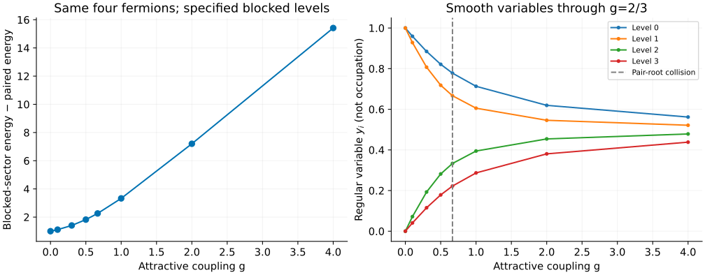
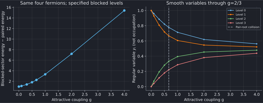
The energy cost of specified blocked levels grows with attraction; regular eigenvalue variables remain smooth at the pair-root collision.

The left panel subtracts the fully paired energy at the same g. The cost is already 1 at g=0 because blocking changes the kinetic occupation. It is not just the lost interaction energy, nor a BCS mean-field gap. The solver does not search over all blocked choices or provide a complete excitation spectrum; call this the cost of the specified blocked sector, not an optimized pair-breaking threshold. The blocked spins' orientations do not affect this Hamiltonian's energy.

The distinction is visible even in trivial limits. Four filled pairs at g=1 have E=12-4=8, not 12. Zero pairs with level 1 blocked have E=1, not zero.

3. Cross a root collision without a physical singularity¶

Richardson pair rapidities can collide with a level pole and become a complex conjugate pair. The implementation follows the regular eigenvalue variables of Faribault et al., rather than those individual rapidities. With \(e_i=2\epsilon_i\) on the L active levels,

\[ \begin{aligned} y_i&=g\sum_{\alpha=1}^{M}\frac1{e_i-E_\alpha},\\{} y_i(y_i-1)-g\sum_{j\ne i}\frac{y_i-y_j}{e_i-e_j}&=0,\qquad \sum_i y_i=M. \end{aligned} \]

The right panel plots these y variables for the two-pair sector. At g=2/3, both pair roots meet the pole at zero, but the regular variables are simply

\[ (y_0,y_1,y_2,y_3)=\left(\frac79,\frac23,\frac13,\frac29\right), \qquad E_{\mathrm{total}}=0. \]

Their defining root sum is interpreted by continuation at the collision. The smooth ground state has not undergone a finite-system phase transition. Above it, the conjugate rapidities still give a real total energy.

These variables are not occupations, despite starting at 1,1,0,0 when g=0. --variables does not reconstruct pair rapidities. Energy is obtained directly from

\[ E=\sum_{i\ \mathrm{active}}2\epsilon_i y_i -gM(L-M+1)+\sum_{i\ \mathrm{blocked}}\epsilon_i. \]

Our tests reconstruct the two roots away from the collision as an independent check, but root reconstruction is not a public frontend capability.

4. Set up an orbital-MPS comparison¶

Use the same single-particle levels, pair number, blocked positions and diagonal i=j interaction. A paired active level has the local states empty and doubly occupied; a blocked fermion is not an empty active level. There is no lattice momentum or PBC/OBC choice for this all-to-all pairing model.

Two inexpensive normalization tests help catch implementation mismatches:

Shifting every single-particle level by a adds \(a(2M+B)\) to E, where B is the number of blocked levels. With four particles and a=5, the shift is 20.
Multiplying all levels and g by a positive factor s multiplies E by s, while leaving y unchanged.

The downloads include both tests, an irregular level spectrum and an analytic two-level case: levels 0,1 with one pair have \(E=1-g-\sqrt{1+g^2}\). Repeated levels/higher degeneracies, repulsive g, generic excited states and form factors are not implemented.

Continuation diagnostics matter. An incomplete run can contain a valid energy at reached_g, not requested_g. The plotting script requires target convergence, matching couplings and acceptable reached/target residuals. A small polynomial residual is not a bound on energy error; clustered levels may require native long-double or optional MPLAPACK fp128.

5. Reproduce and validate¶

Each link is a native export with provenance and convergence diagnostics:

g	Two pairs: state / variables	One pair, blocked 1,2: state / variables
0	state / variables	state / variables
0.1	state / variables	state / variables
0.3	state / variables	state / variables
0.5	state / variables	state / variables
2/3	state / variables	state / variables
1	state / variables	state / variables
2	state / variables	state / variables
4	state / variables	state / variables

Check	State	Variables
Two levels, one pair	CSV	CSV
All levels paired	CSV	CSV
No pairs, one blocked fermion	CSV	CSV
Free, with a blocked fermion	CSV	CSV
Shifted levels	CSV	CSV
Energy scaling	CSV	CSV
Irregular levels	CSV	CSV
Reversed blocked-index order	CSV	CSV
Weak coupling	CSV	CSV

With the plotting dependencies, from the source checkout:

python3 scripts/plot_gaudin_tutorial.py --check
python3 scripts/plot_gaudin_tutorial.py
# Optional: regenerate both Gaudin-model tutorials.
python3 scripts/plot_gaudin_tutorial.py --solver-dir /path/to/bethe/bin
# Optional independent occupation/spin matrices; requires NumPy.
python3 scripts/plot_gaudin_tutorial.py --check --oracle
python3 -m unittest discover -s scripts -p 'test_tutorial_gaudin.py'

The script validates all input indices, blocked nulls, equations, number constraints and reconstructed energies before saving regenerated data. The optional matrix oracle compares every saved sector with the smallest eigenvalue of its independent occupation-space Hamiltonian. Tests cover the collision, original pair equations, exact limits and dishonest incomplete/corrupted exports.