Lieb–Liniger: particle and hole branches¶

View this page on GitHub

What happens to the excitation spectrum of a one-dimensional Bose gas as repulsion increases? This tutorial plots the two Lieb branches, then changes the density to show which parts of a comparison are physics and which are units. The results are useful benchmarks for continuum MPS calculations or for a lattice discretization approaching the continuum limit.

We use the zero-temperature, repulsive gas on an infinite line. The reference guide gives the integral equations; the finite-ring guide covers individual finite-size states.

1. Fix the units before choosing a coupling¶

The Hamiltonian and dimensionless interaction are

\[ H=-\sum_j\partial_{x_j}^2+2c\sum_{i\lt j}\delta(x_i-x_j), \qquad n=N/L,\qquad \gamma=c/n,\qquad c\gt0. \]

Here \(\hbar=2m=1\). The number supplied to --c is not the dimensionless interaction unless the density is one. Momentum has units of inverse length and energy of inverse length squared. There is no lattice Brillouin zone.

For a build containing bethe-lieb-liniger-dispersion, start with:

bethe-lieb-liniger-dispersion --c 1 --density 1 --points 129
bethe-lieb-liniger-dispersion --c 1 --density 1 --points 129 \
  --precision fp64 --format csv > ll-c1-n1.csv

The CSV includes the background solution, numerical status and provenance as comments. Its energy column contains fixed-particle-number excitation gaps, not total energies and not particle-addition energies. Do not add a chemical potential to these curves.

2. Two ways to excite the Bethe sea¶

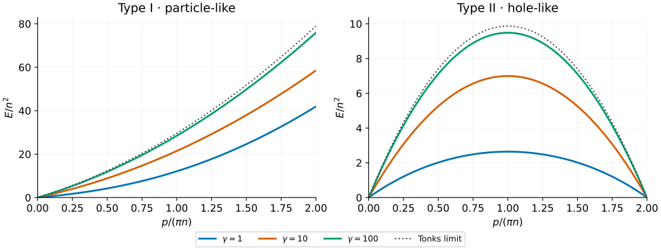
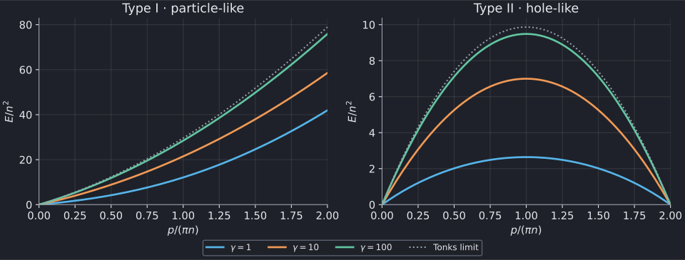
Type-I and type-II spectra at three repulsions, with the Tonks limiting curves

The coloured curves are solver exports at \(n=1\): c = 1, c = 10 and c = 100.

Type I: move a particle from the right edge of the occupied rapidity sea to a rapidity outside it. The physical momentum starts at zero and is unbounded. The right edge of this plot is only a plotting cutoff.
Type II: make a hole inside the sea and put the particle at the right edge. Its momentum runs from zero to \(2\pi n\), with a maximum energy at \(\pi n\) and zero energy at both endpoints.

Both processes keep \(N\) fixed. “Particle” and “hole” describe rearrangements of Bethe rapidities, not a change of bosonic statistics. The exported rapidity is also not the physical momentum p.

The dotted curves are explicitly analytic limiting references, not extra solver data. In the impenetrable, or Tonks–Girardeau, limit:

\[ E_{\mathrm I}(p)=p(2\pi n+p),\qquad E_{\mathrm{II}}(p)=p(2\pi n-p). \]

The finite-coupling curves approach these limits as \(\gamma\) grows; even \(\gamma=100\) is not the limit itself. At smaller coupling the type-II branch lies much lower, making it a particularly useful test of an excitation calculation beyond a simple particle-like approximation.

To extend only the type-I grid, choose a larger physical momentum cutoff:

bethe-lieb-liniger-dispersion --c 1 --density 1 --p-max 12 --points 257

Why is there a second zero without momentum periodicity?¶

On a ring, boosting every particle by \(2\pi/L\) gives a total momentum \(2\pi n\) but an energy cost \(4\pi^2 n/L\) above the zero-momentum ground state. That cost vanishes in the thermodynamic limit. This explains the second type-II zero; it does not identify momenta modulo \(2\pi n\) or make the unbounded type-I branch periodic.

3. Double the density without changing the dimensionless problem¶

Compare \((c,n)=(1,1)\) with \((2,2)\). Both have \(\gamma=1\).

bethe-lieb-liniger-dispersion --c 2 --density 2 --points 129 \
  --precision fp64 --format csv > ll-c2-n2.csv

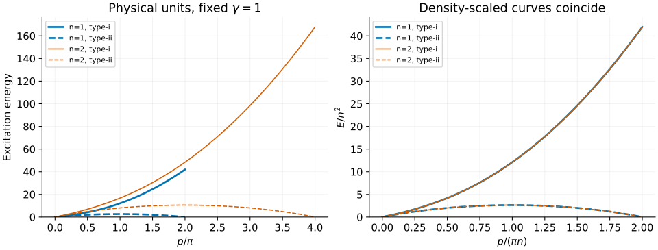
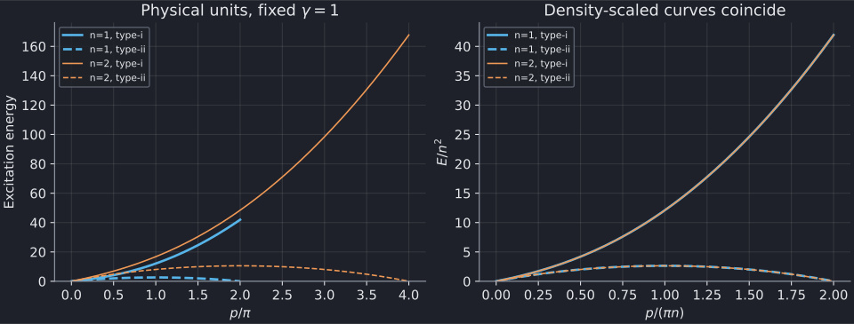
Physical spectra change with density, but scaled spectra coincide

The left panel uses physical units; the right plots the same data using \(p/(\pi n)\) and \(E/n^2\). Both branches collapse. Download the second-density export to check this directly.

At fixed \(\gamma\), the scaling rules are:

Exported quantity	Density dependence
Momentum and Fermi rapidity	\(n\)
Excitation energy and chemical potential	\(n^2\)
Ground energy per length	\(n^3\)

Confusing energy per length with energy per particle introduces an extra factor of density. The tutorial tests check all three powers, not only the visual collapse.

4. Comparing with an excitation ansatz¶

Match the kinetic-energy coefficient, density and \(c/n\) first. For a lattice approximation, convert lattice momentum and energy using the lattice spacing before taking a continuum limit. A finite-spacing lattice dispersion is not expected to match an unbounded continuum curve at arbitrary momentum.

These lines supply energies, not spectral weights. This figure does not shade or enumerate a complete multiparticle continuum. A visible numerical branch and a strong peak in a particular correlation function are different claims.

Check the background and each row's status before plotting. A failed mesh or momentum inversion is not a zero-energy excitation. The default fp64 data are adequate for these examples; --precision long-double and --precision fp128 are available when supported by the build. Very small \(\gamma\) may require larger numerical meshes as well as additional precision.

5. Reproduce the figures¶

Install the optional plotting dependencies as in the first tutorial, then run:

python3 scripts/plot_lieb_liniger_tutorial.py
# Regenerate the four exports with your chosen executable as well:
python3 scripts/plot_lieb_liniger_tutorial.py \
  --solver bethe-lieb-liniger-dispersion
python3 scripts/plot_lieb_liniger_tutorial.py --check
python3 -m unittest discover -s scripts -p 'test_tutorial_lieb_liniger.py'

The script validates schemas, conventions, convergence and momentum grids. The tests also check type-II reflection symmetry, the approach to the Tonks limit and density scaling. Plotting reads the saved frontend exports; only the labelled Tonks reference curves use analytic formulas.